The random nature of radioactive decay
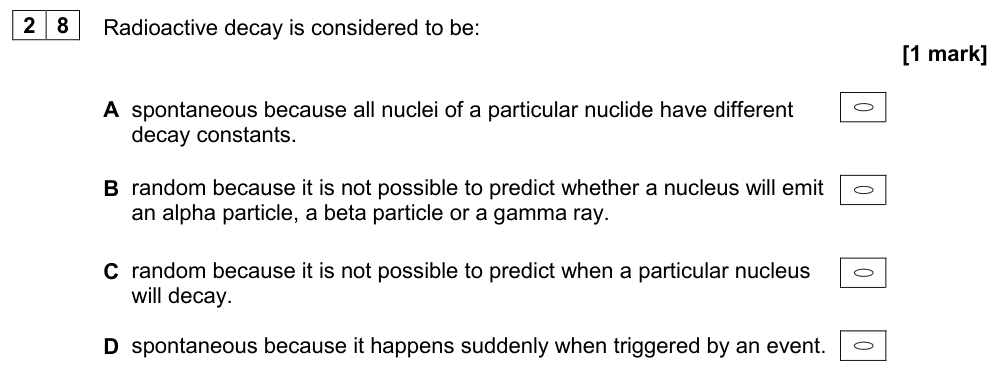
Radioactive decay is random and spontaneous:
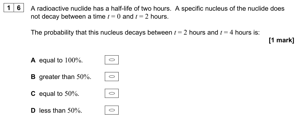
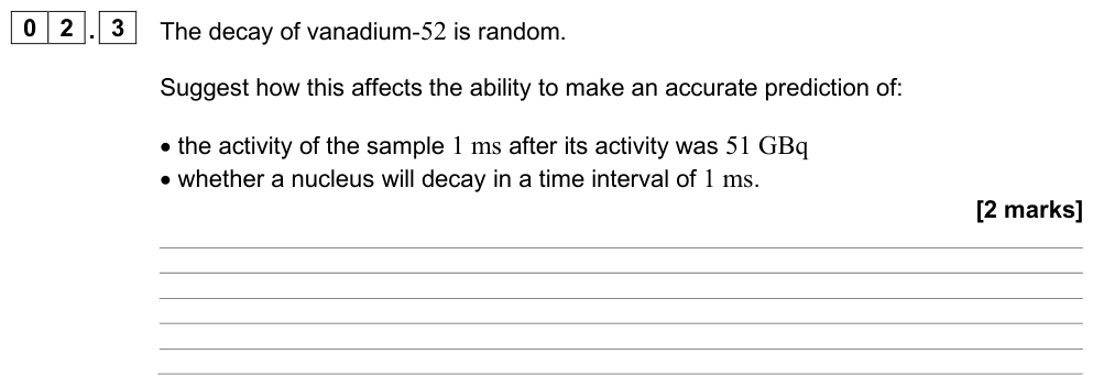
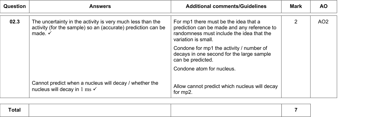
- Random: it is impossible to predict which nucleus will decay next or when a particular nucleus will decay.
- Spontaneous: decay is not affected by external factors such as temperature, pressure or chemical bonding.
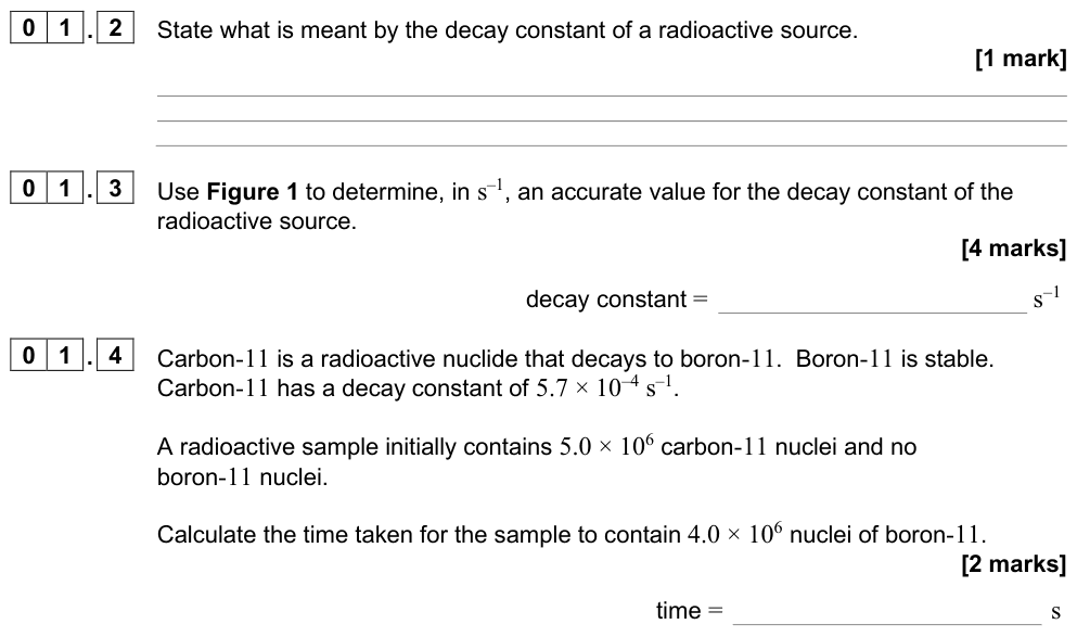
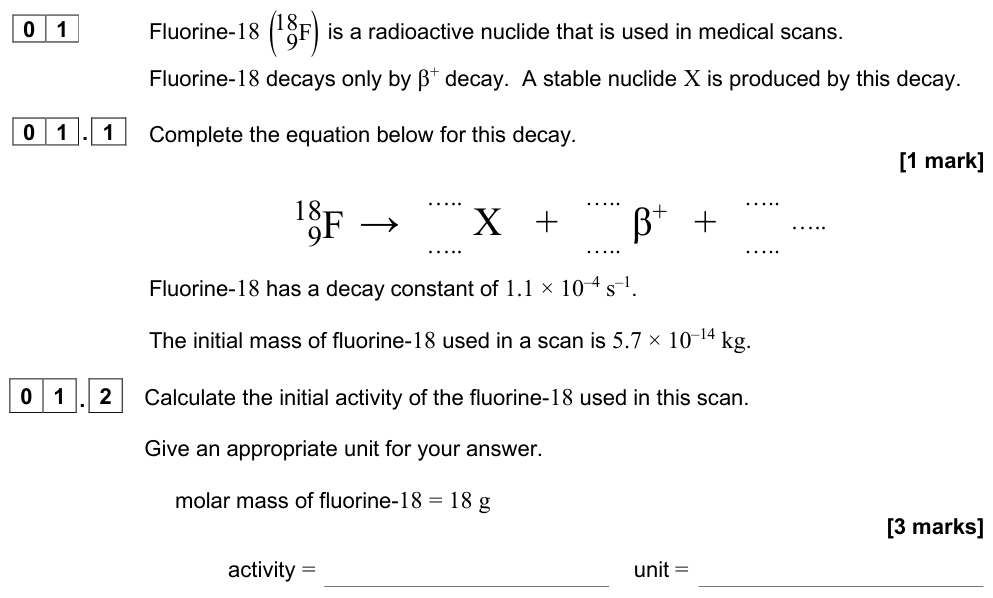
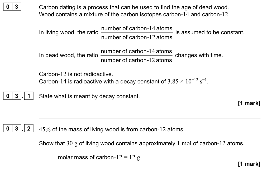
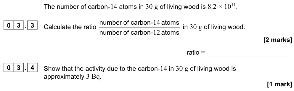
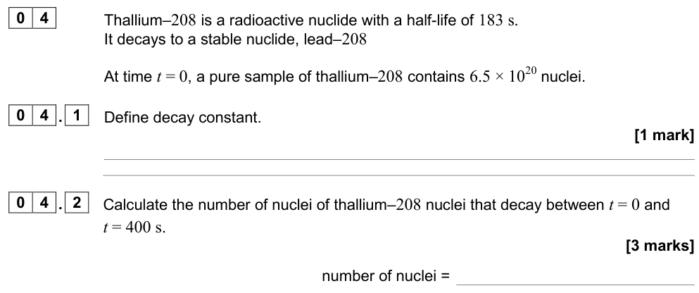
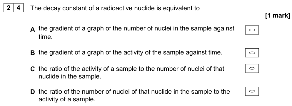
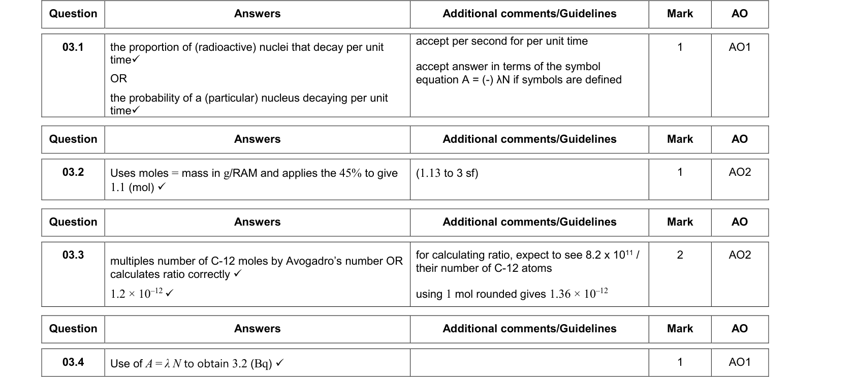
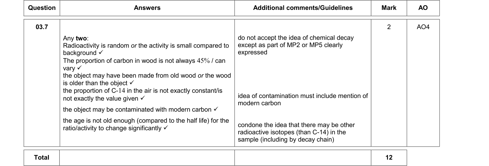
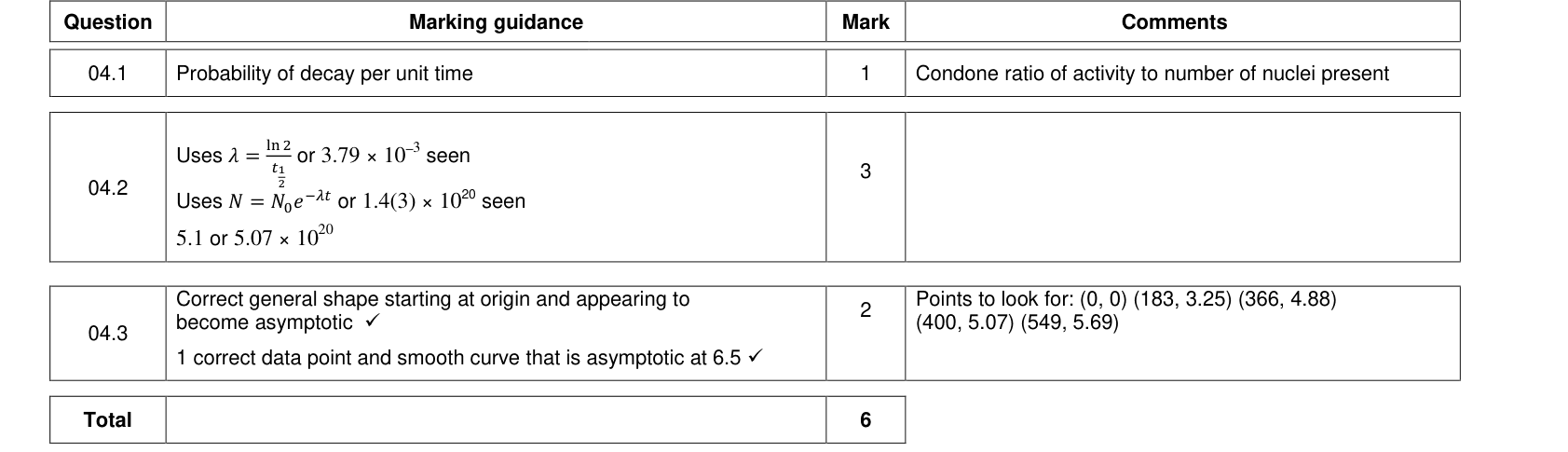
However, every nucleus of a given nuclide has the same constant probability of decaying per unit time. This probability is the decay constant $\lambda$ (unit s⁻¹). With a very large number of nuclei, the behaviour of the sample as a whole is entirely predictable.
The decay equation
The number of nuclei decaying per second is proportional to the number of undecayed nuclei present:
Rate of decay
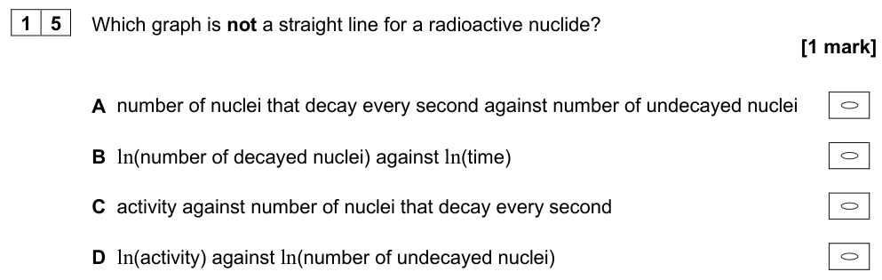
$$\frac{\Delta N}{\Delta t} = -\lambda N$$
The minus sign shows that $N$ decreases.
This leads to exponential decay:
Exponential decay
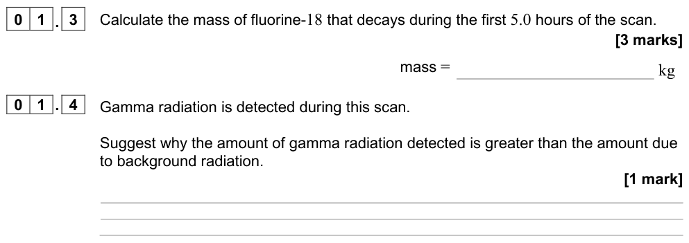
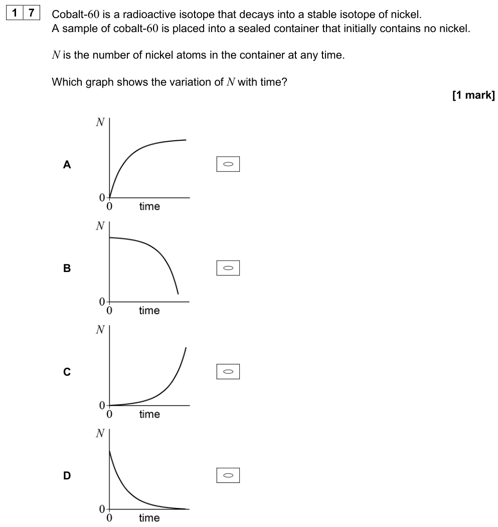
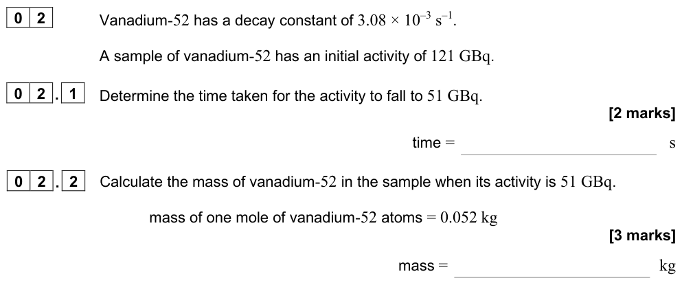
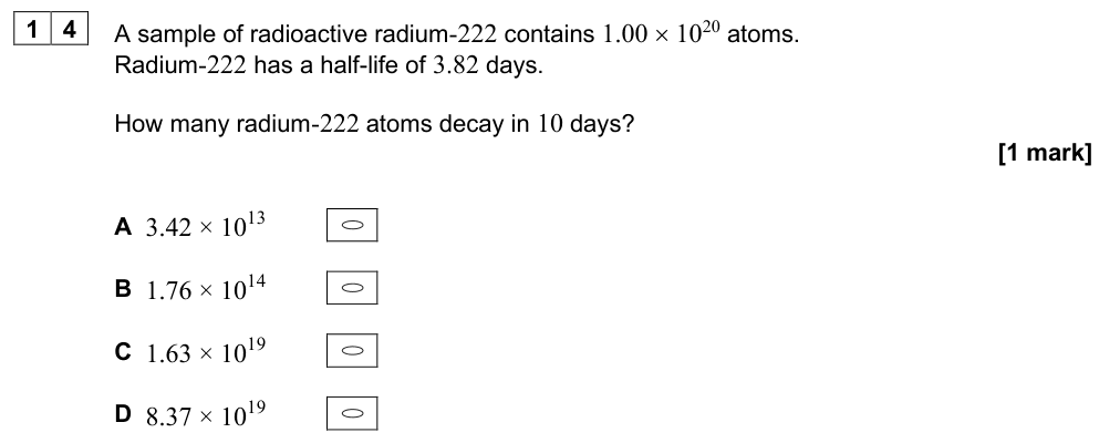
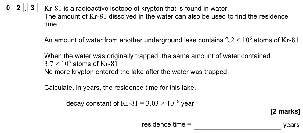
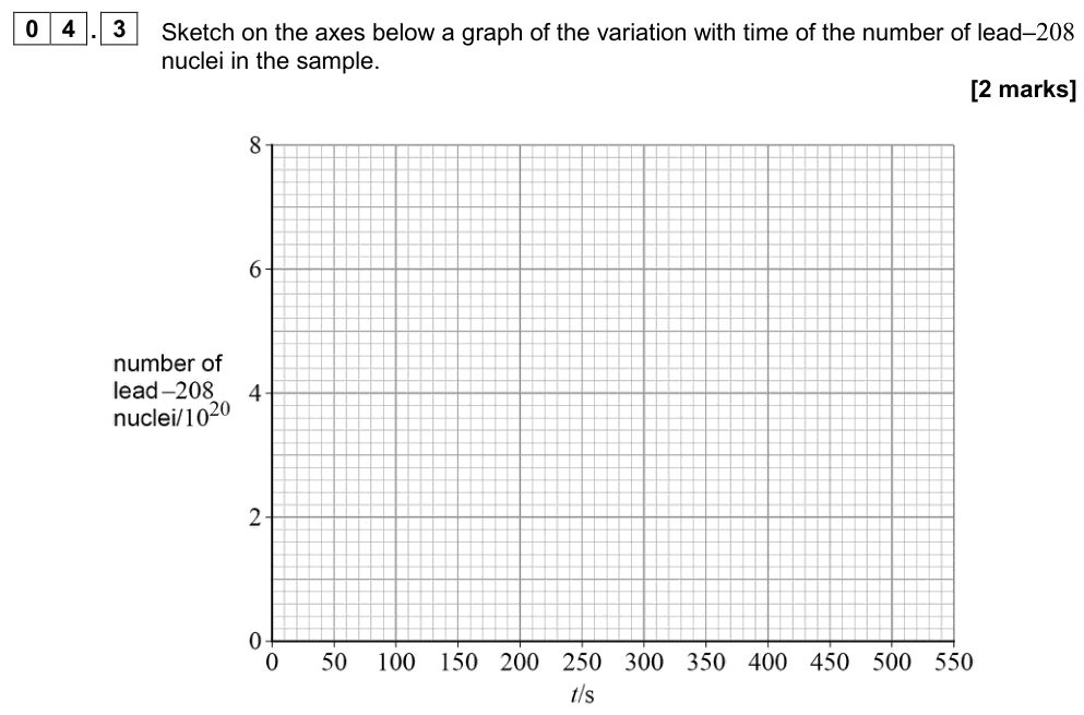
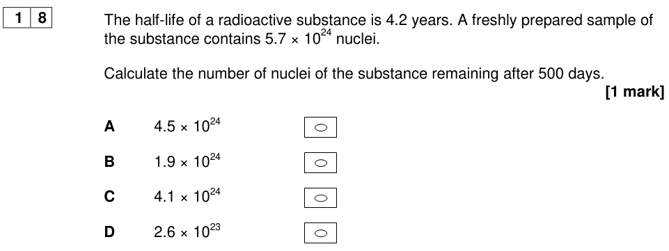
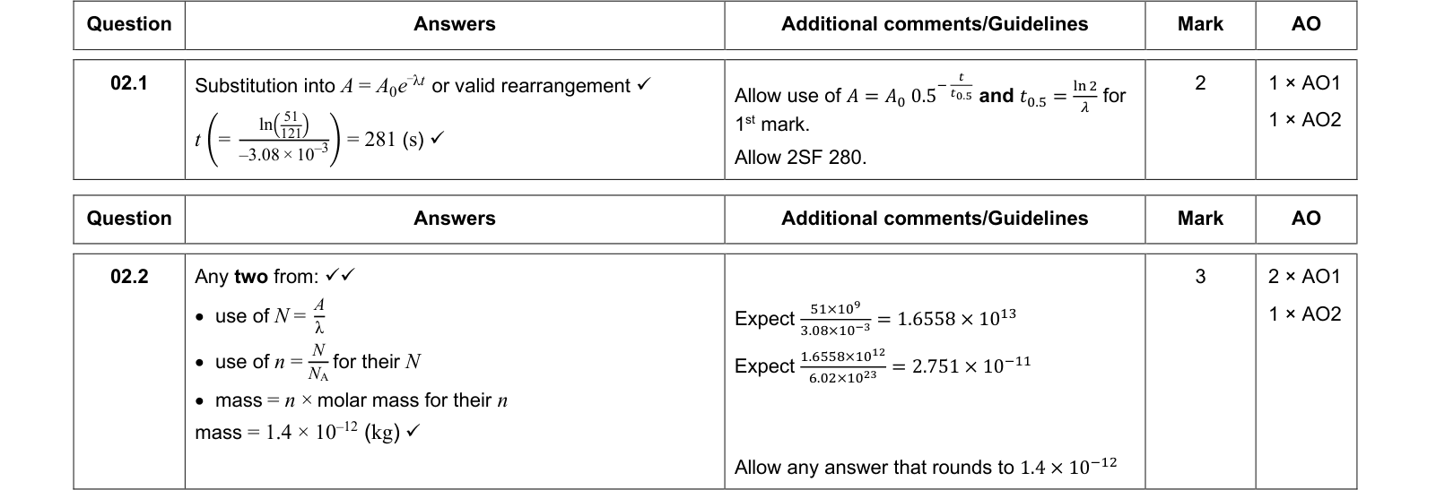
$$N = N_0e^{-\lambda t}$$
$N_0$ = initial number of undecayed nuclei; $N$ = number remaining after time $t$.
Activity
Activity
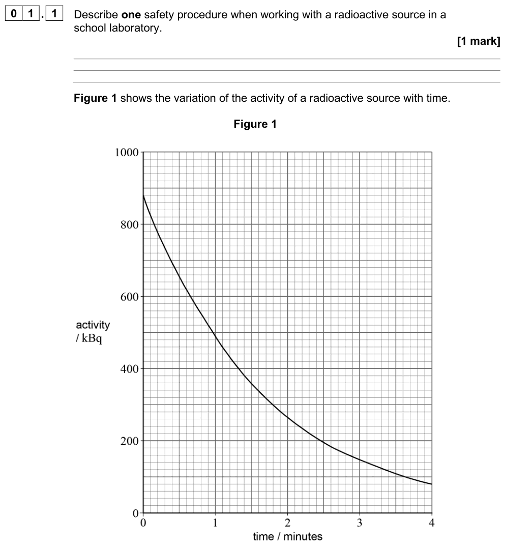
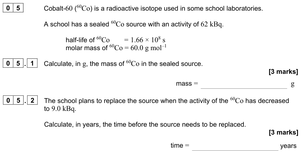
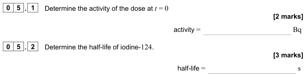
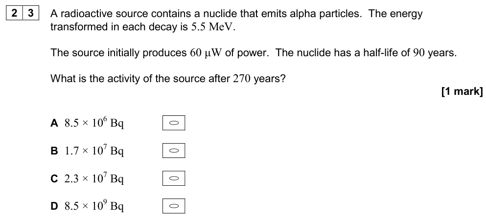
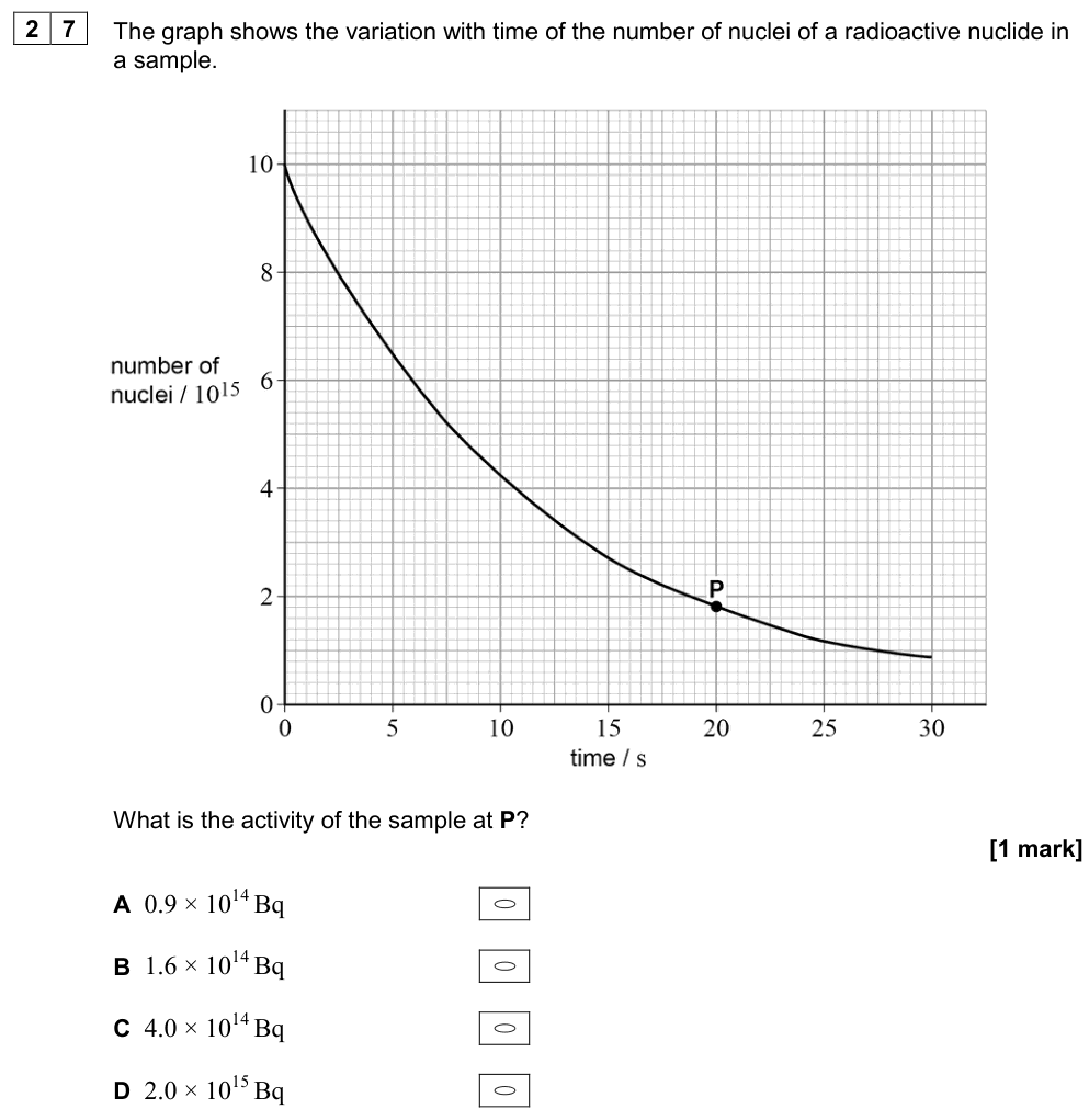
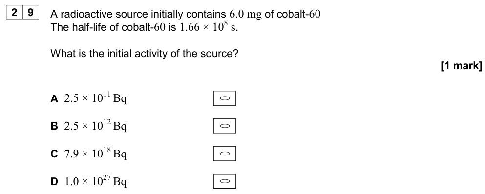
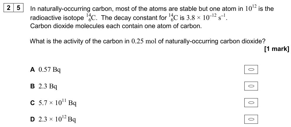
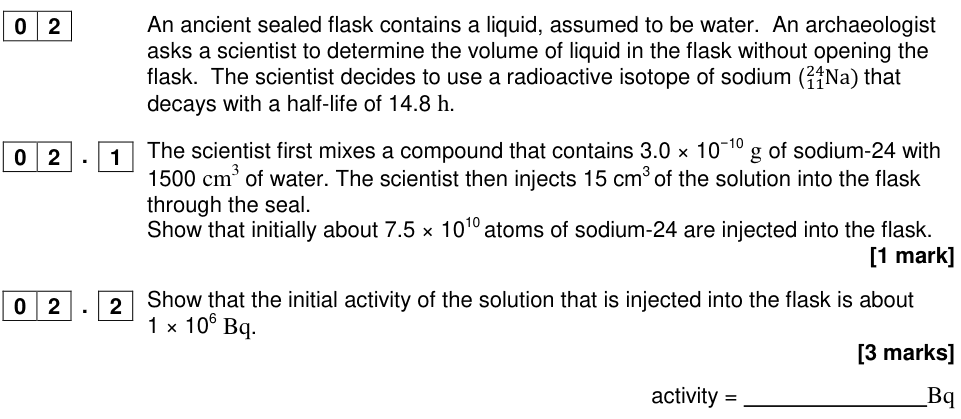
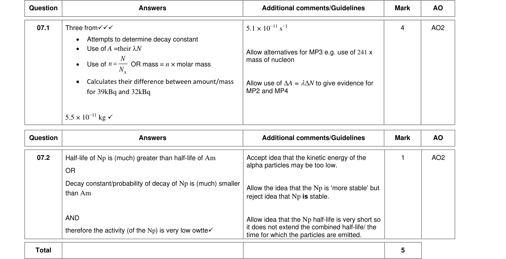
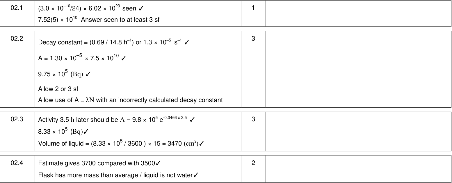
The activity $A$ of a sample is the number of nuclei decaying per second. Unit: becquerel (Bq); 1 Bq = 1 decay per second.
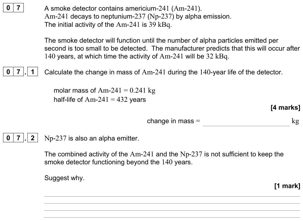
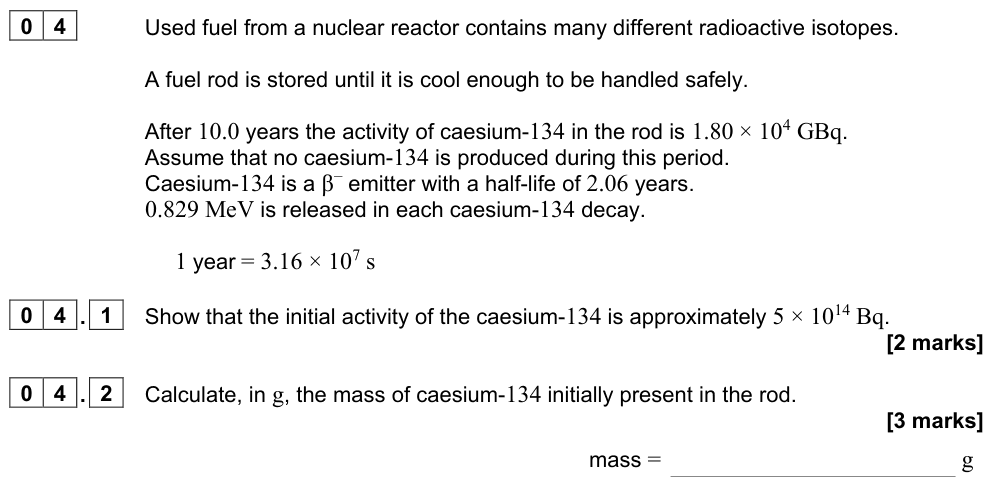
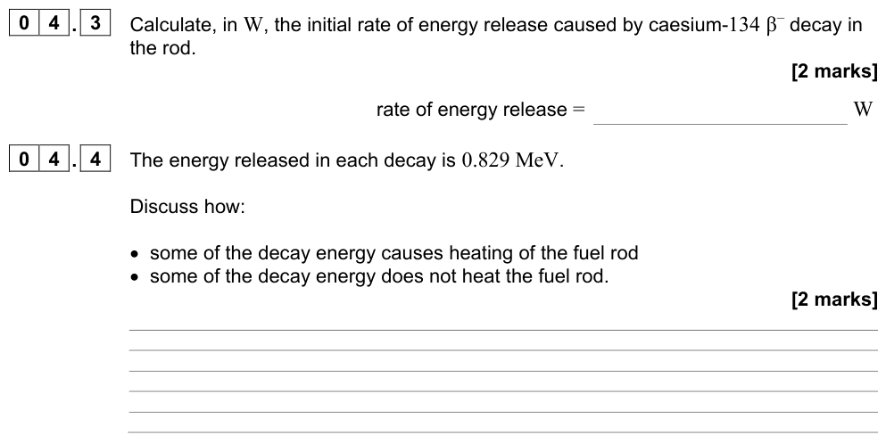
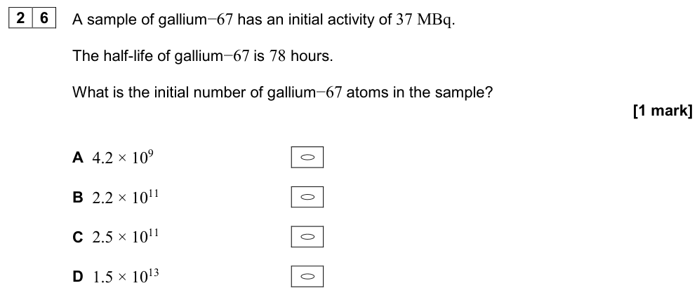
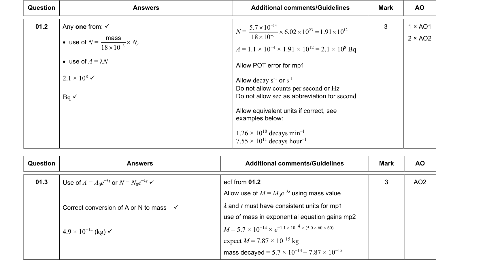
$$A = \lambda N \qquad A = A_0e^{-\lambda t}$$
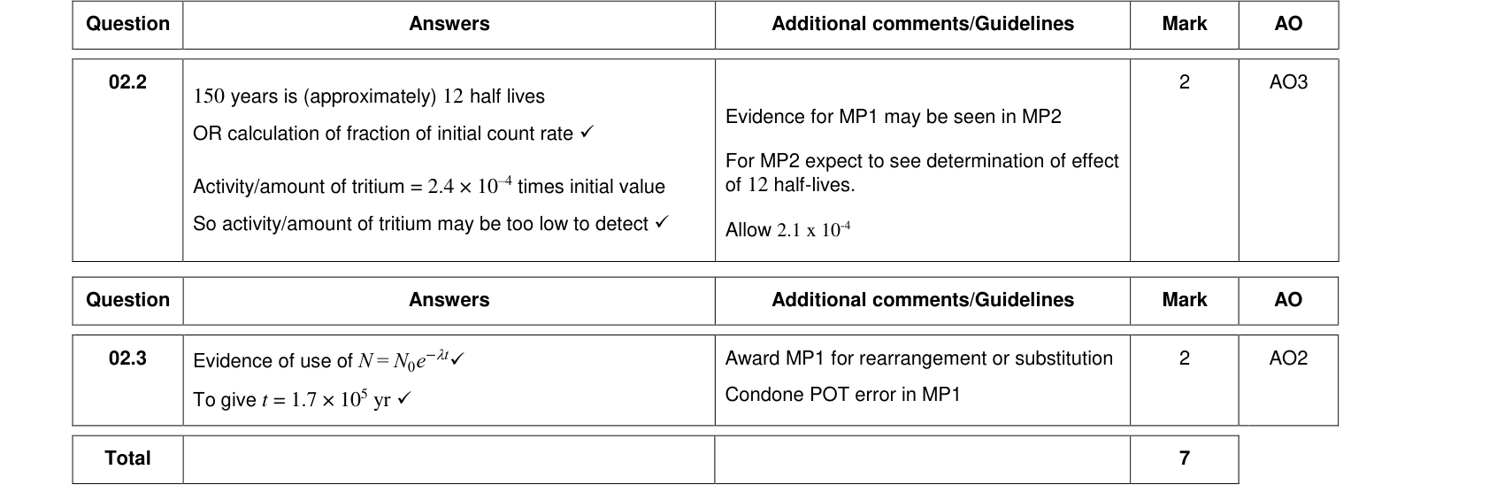
The activity is proportional to the number of undecayed nuclei, so it decays with the same half-life. The count rate measured by a detector is proportional to the activity (only a fraction of the emissions enter the detector) and also decays exponentially, once background is subtracted.
Half-life
Half-life
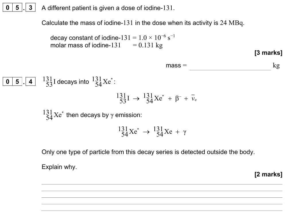
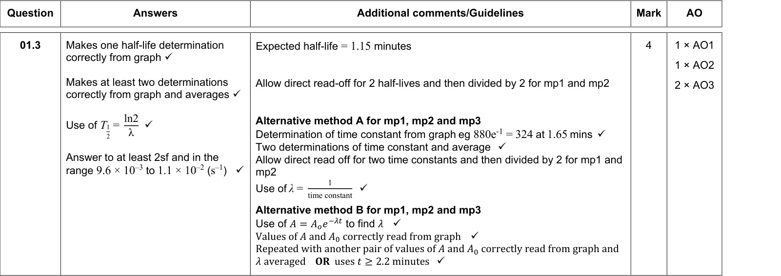
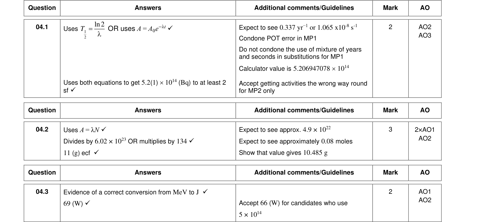
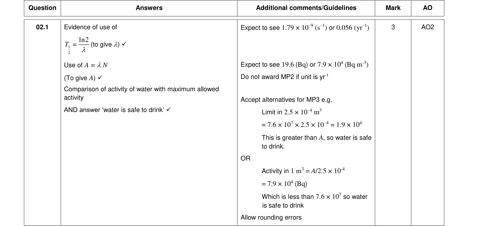
$$T_{1/2} = \frac{\ln2}{\lambda} = \frac{0.693}{\lambda}$$
Derivation: after one half-life $N = \tfrac12N_0$, so $\tfrac12 = e^{-\lambda T_{1/2}}$, giving $\lambda T_{1/2} = \ln 2$.
A short half-life means a large decay constant: the nuclide decays quickly and, for a given number of nuclei, has a high activity.
Worked example: activity of a sample
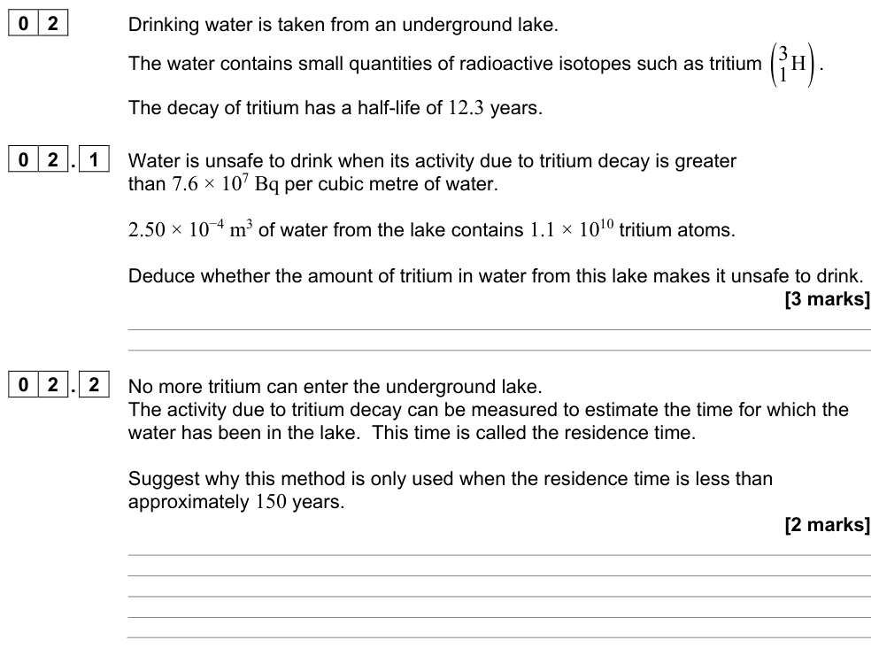
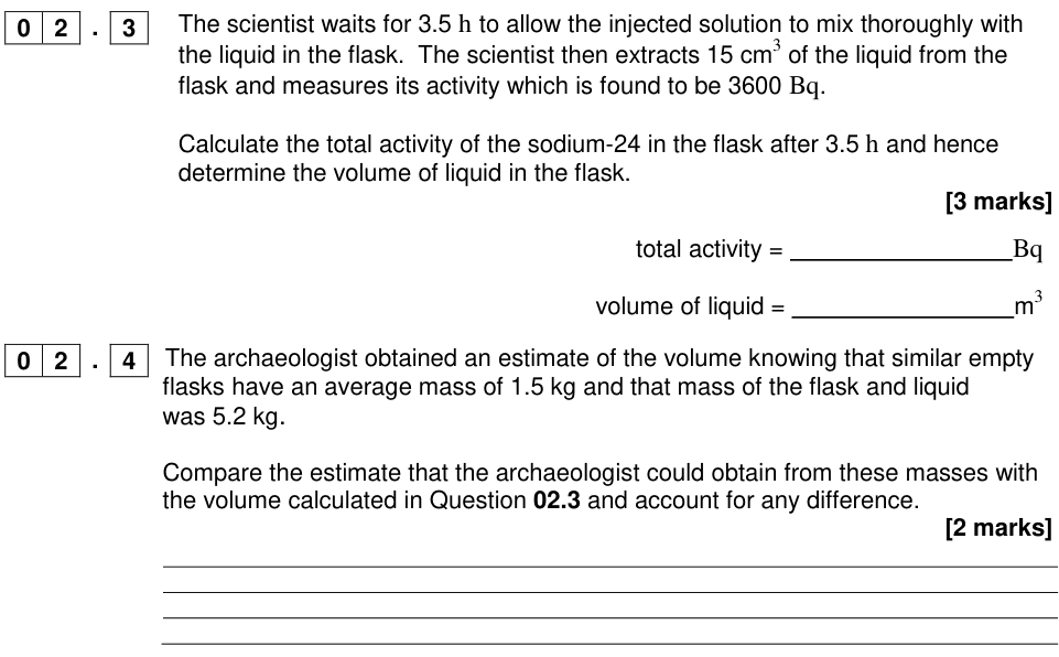
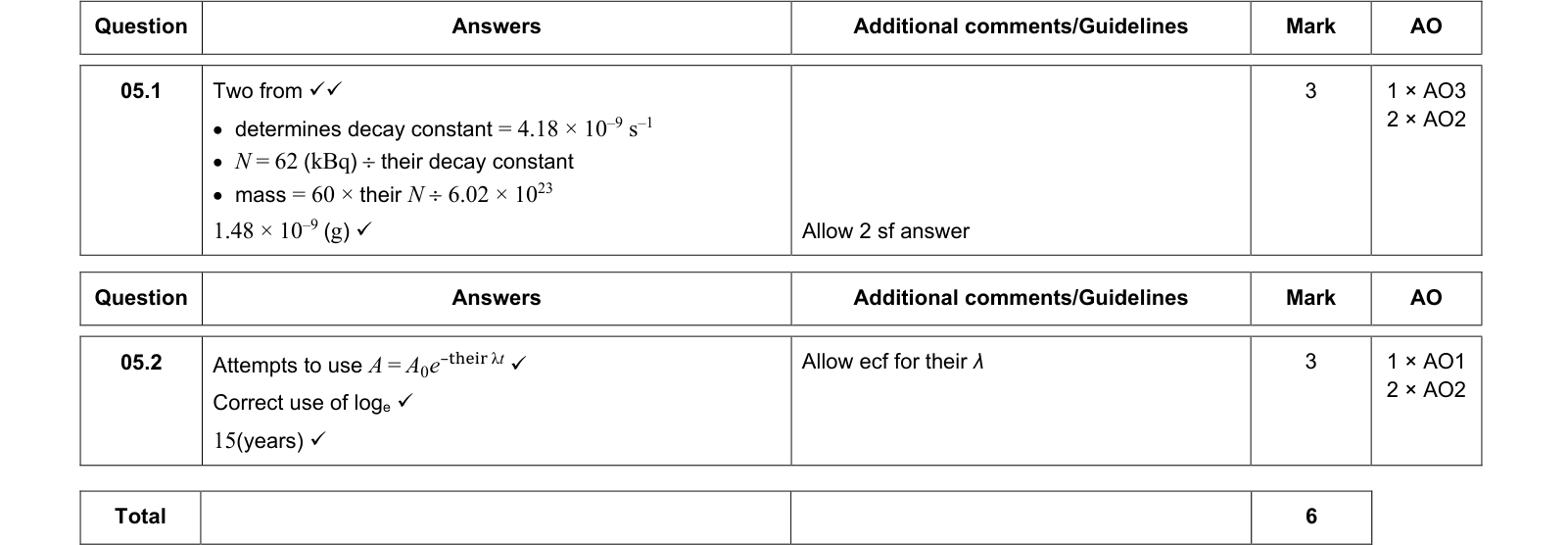
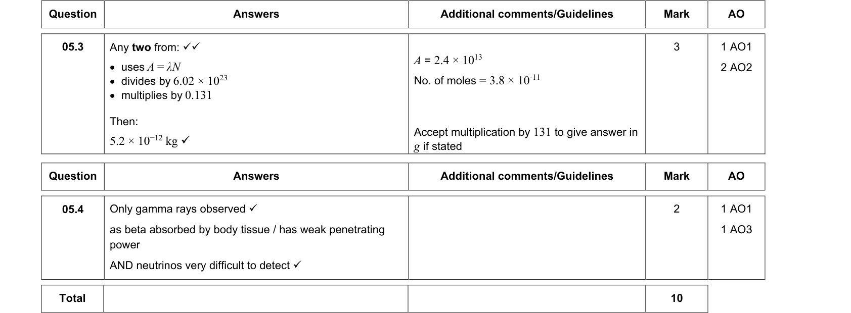
Cobalt-60 has a half-life of 5.27 years. Find the activity of 1.0 μg of cobalt-60.
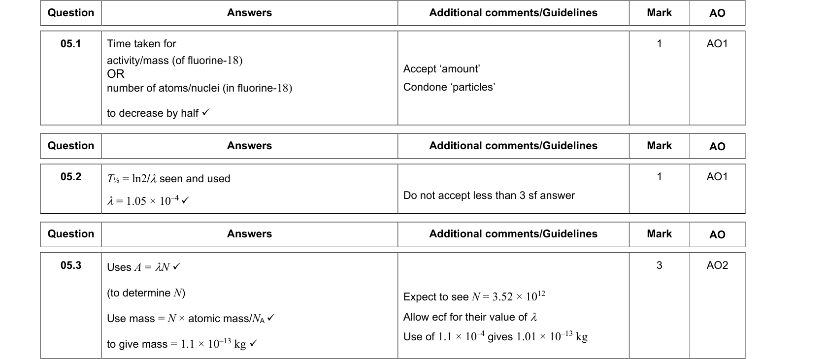
$\lambda = \dfrac{0.693}{5.27 \times 3.15 \times 10^{7}} = 4.17 \times 10^{-9}\ \text{s}^{-1}$.
Number of nuclei: $N = \dfrac{1.0 \times 10^{-6}\ \text{g}}{60\ \text{g mol}^{-1}} \times 6.02 \times 10^{23} = 1.00 \times 10^{16}$.
$A = \lambda N = 4.2 \times 10^{7}\ \text{Bq}$.
Using molar mass and the Avogadro constant
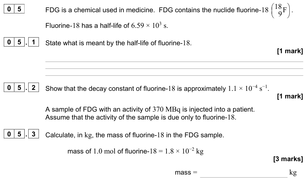
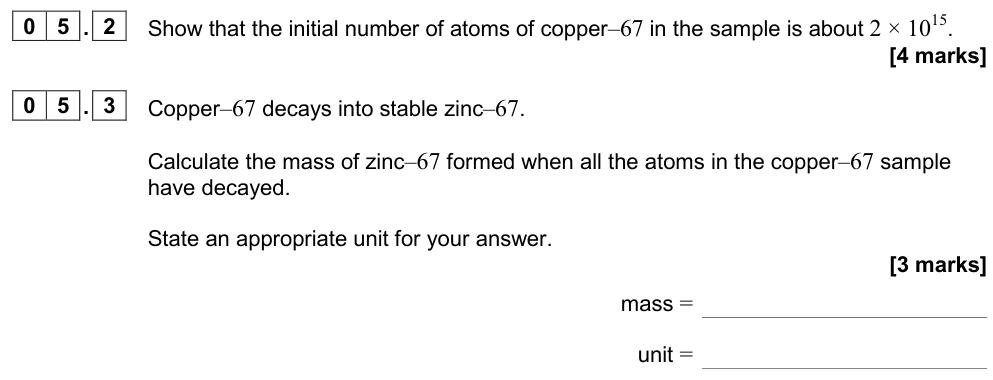
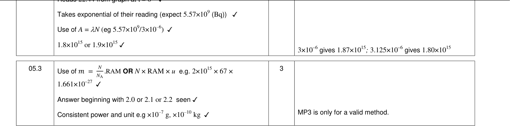
$$N = \frac{\text{mass}}{\text{molar mass}} \times N_A$$
Make sure the mass and molar mass are in the same units (g and g mol⁻¹, or kg and kg mol⁻¹). $N_A = 6.02 \times 10^{23}\ \text{mol}^{-1}$.
Worked example: carbon dating
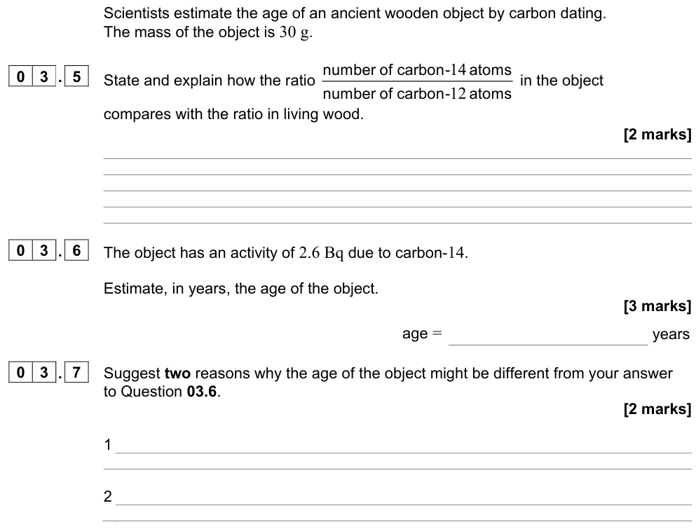
Living wood has an activity of 0.25 Bq per gram from carbon-14 ($T_{1/2} = 5730$ years). An ancient sample has 0.080 Bq per gram. How old is it?
$\lambda = 0.693/5730 = 1.21 \times 10^{-4}\ \text{y}^{-1}$.
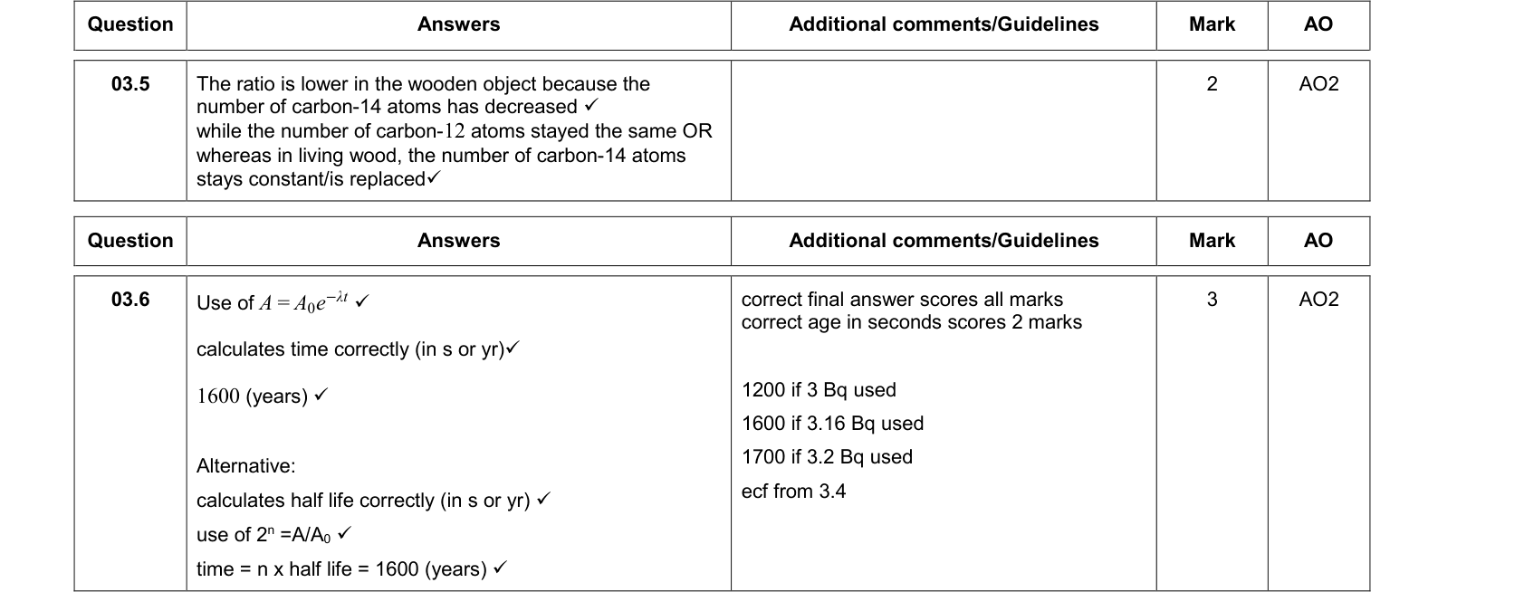
$0.080 = 0.25e^{-\lambda t} \Rightarrow t = \dfrac{\ln(0.25/0.080)}{1.21 \times 10^{-4}} = 9400$ years.
Common mistake
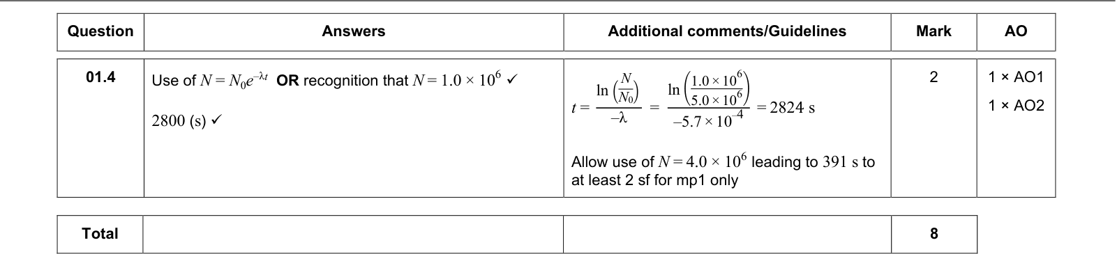
Keep units consistent: if $\lambda$ is in s⁻¹, $t$ must be in seconds. The half-life can be in any time unit as long as $t$ is in the same unit.
Determining half-life from data
From a decay curve
Plot the (corrected) activity or count rate against time. Read off the time taken to fall from any value to half that value. Repeat from several starting points and take the mean.
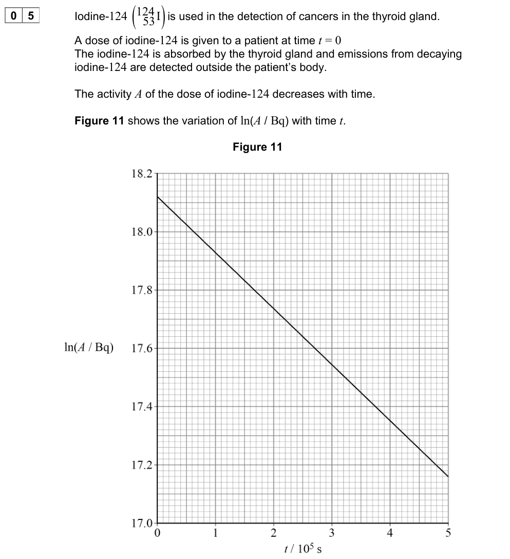
From a log graph
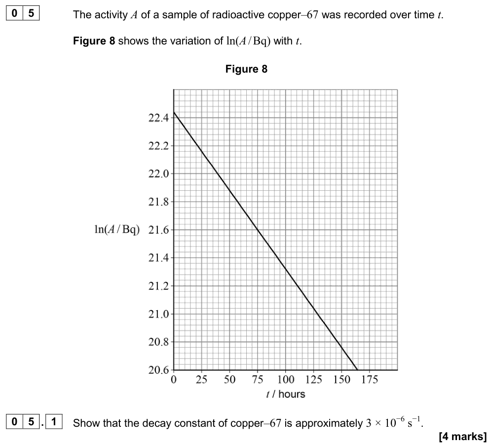
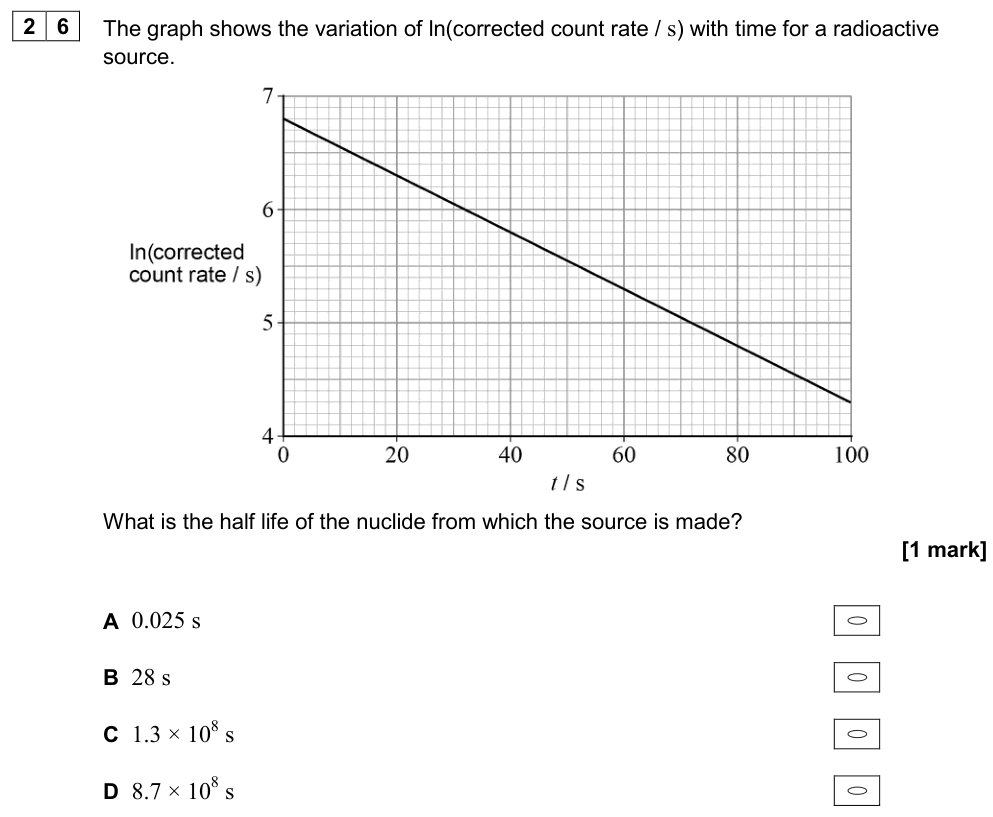
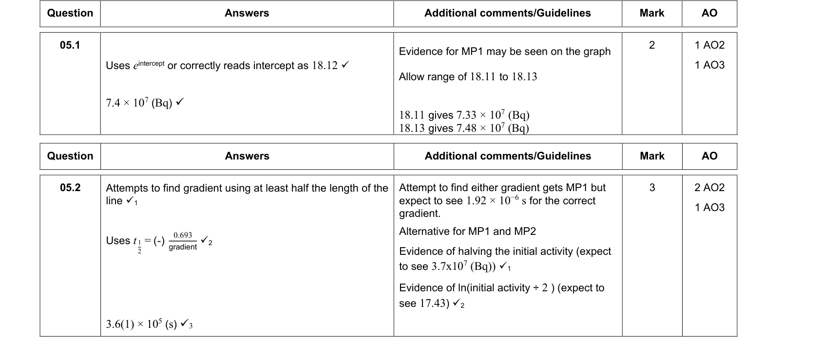
Taking natural logs of $A = A_0e^{-\lambda t}$:
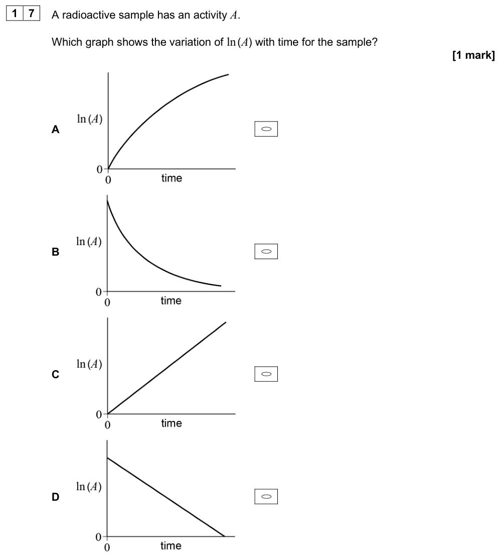
$$\ln A = \ln A_0 - \lambda t$$
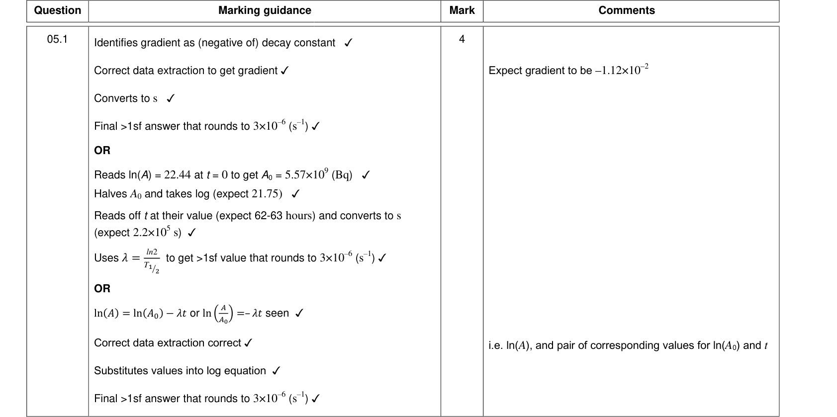
A graph of $\ln A$ (or $\ln$ of the corrected count rate) against $t$ is a straight line with gradient $= -\lambda$ and y-intercept $\ln A_0$. Then $T_{1/2} = \ln2/\lambda$. The log graph uses all the data, averages out random fluctuations and confirms that the decay is exponential.
Worked example
A graph of $\ln(C/\text{s}^{-1})$ against $t$/hours has gradient $-0.0866\ \text{h}^{-1}$. $\lambda = 0.0866\ \text{h}^{-1}$, so $T_{1/2} = 0.693/0.0866 = 8.0$ hours.
Modelling with constant decay probability
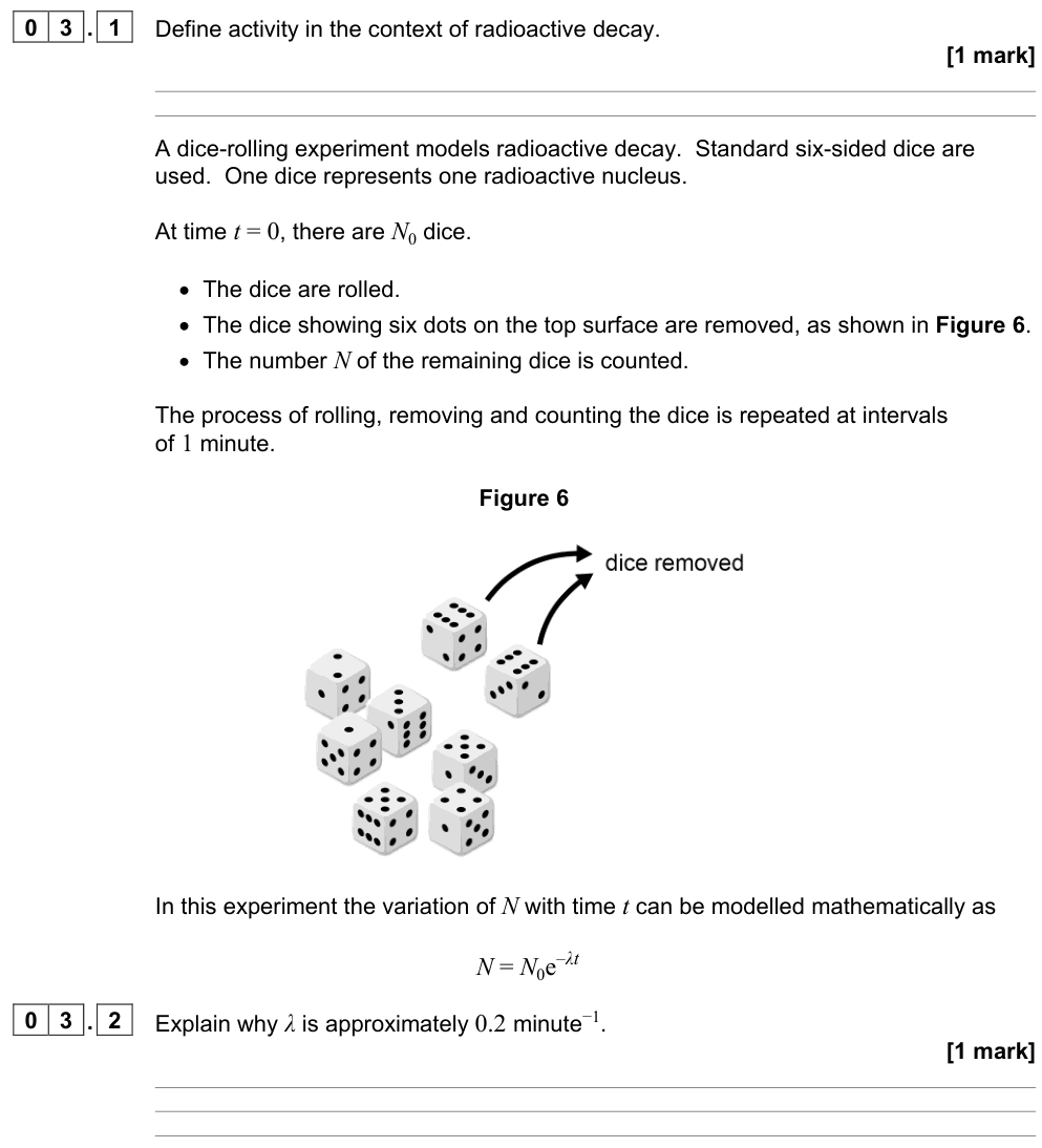
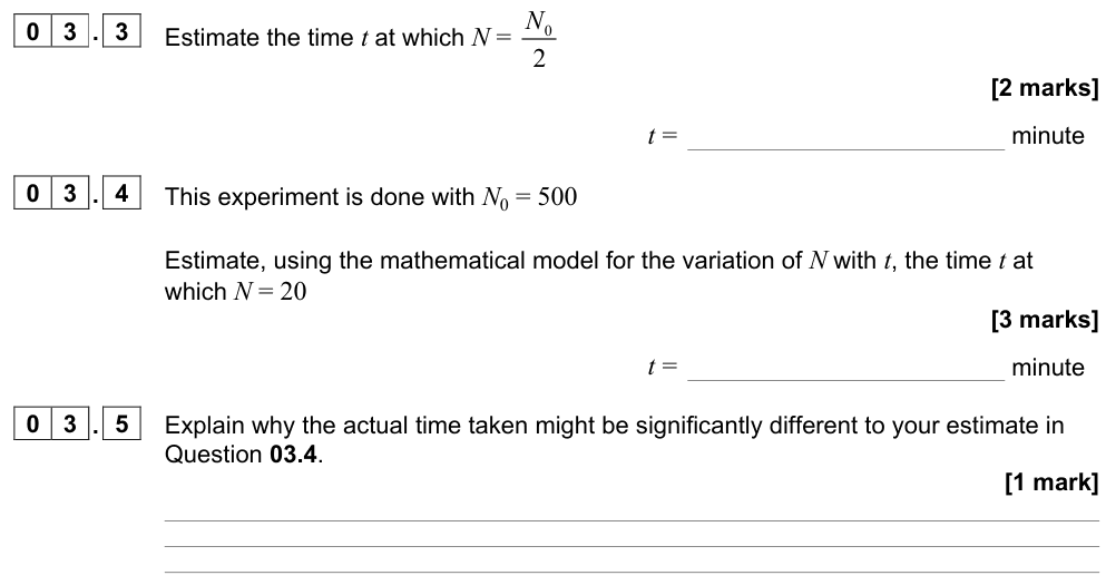
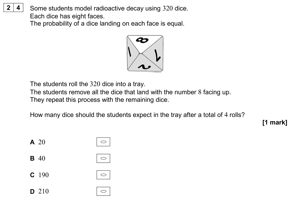
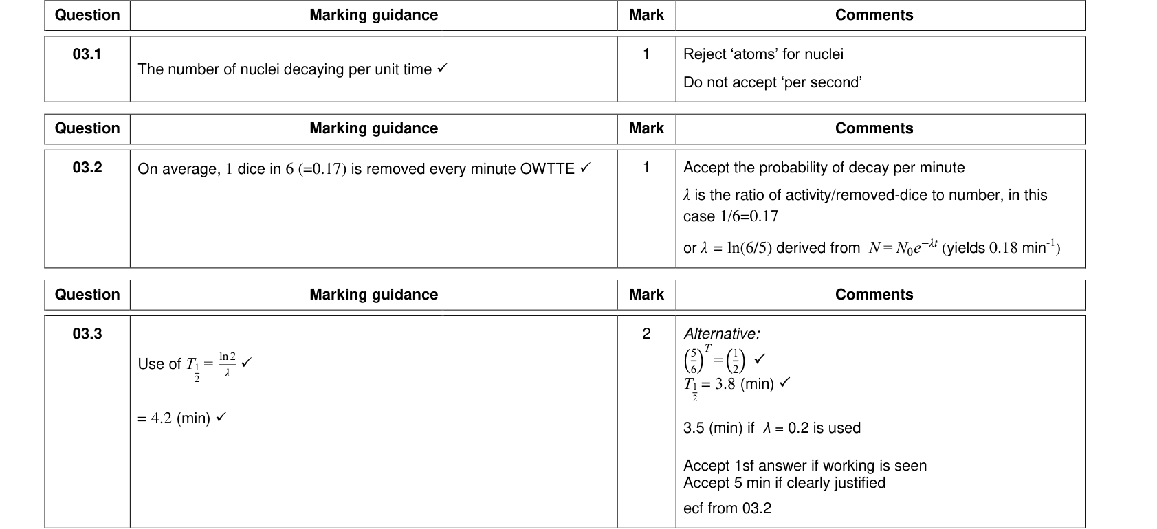
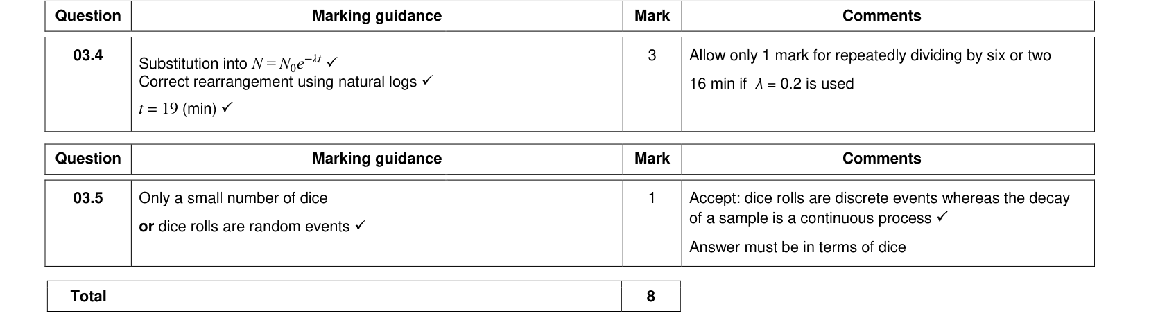
Decay can be modelled with dice. Start with, say, 500 dice. Throw them all; remove every die showing a six (each die has a probability $\tfrac16$ of "decaying" per throw). Count the remaining dice and repeat.
- The number removed each throw is roughly proportional to the number remaining.
- A graph of dice remaining against number of throws is an exponential decay curve.
- The "half-life" is about $\ln2/\lambda = 0.693/(1/6) \approx 4.2$ throws (more precisely $\ln2/\ln(6/5) = 3.8$ throws, because the probability per throw is not small).
- Random scatter is larger when few dice remain, just as count rates fluctuate more at low activity.
The Random decay diagram in the Interactive tab runs this model.
Summary
- Decay is random and spontaneous; each nucleus has a constant decay probability $\lambda$ per second.
- $\Delta N/\Delta t = -\lambda N$; $N = N_0e^{-\lambda t}$; $A = \lambda N = A_0e^{-\lambda t}$.
- $T_{1/2} = \ln2/\lambda$.
- $N = (\text{mass}/\text{molar mass}) \times N_A$.
- $\ln A$ against $t$: straight line, gradient $-\lambda$.