The Young modulus
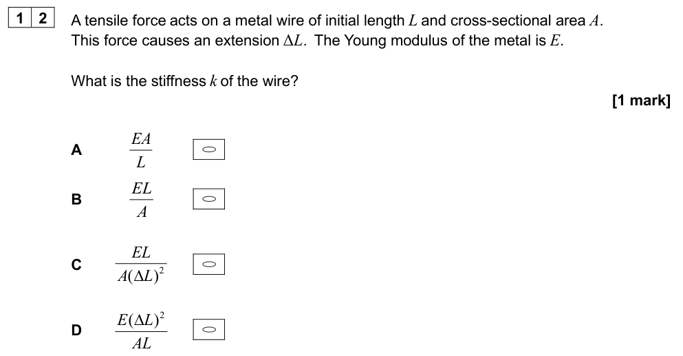
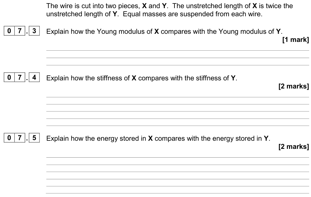
The spring constant $k$ describes a particular object. To describe the stiffness of a material we use the Young modulus, which does not depend on the length or thickness of the sample.
Young modulus
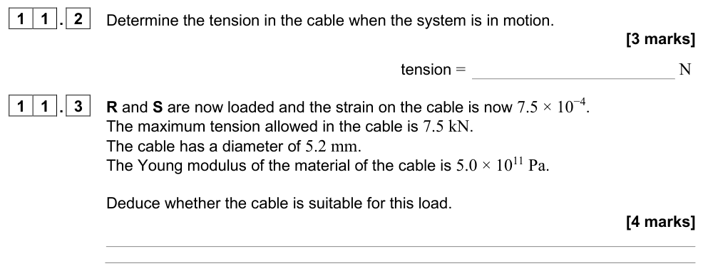
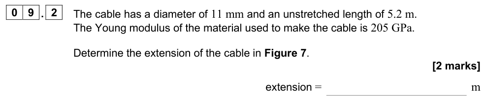
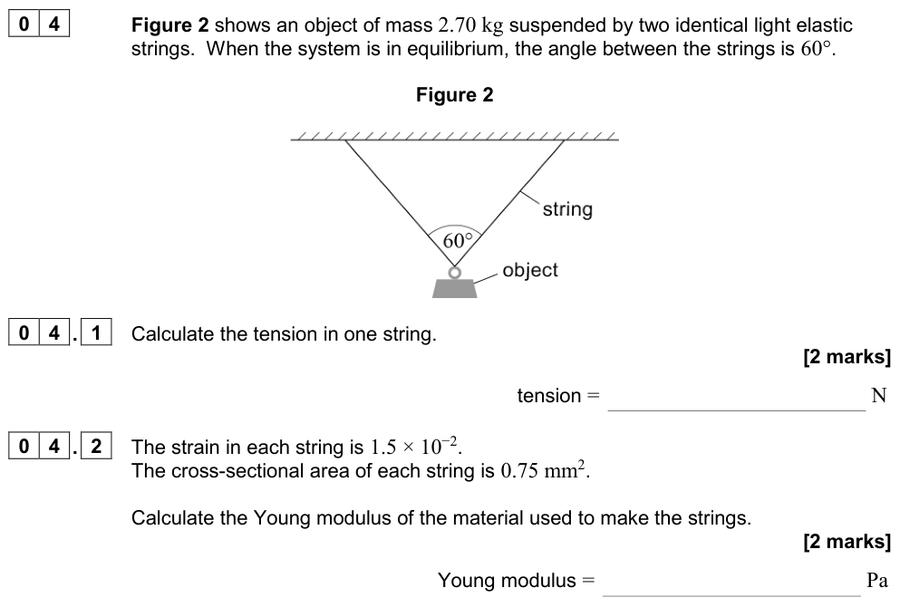
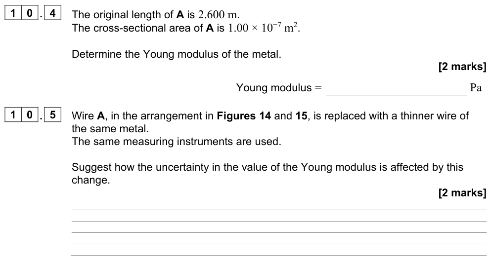
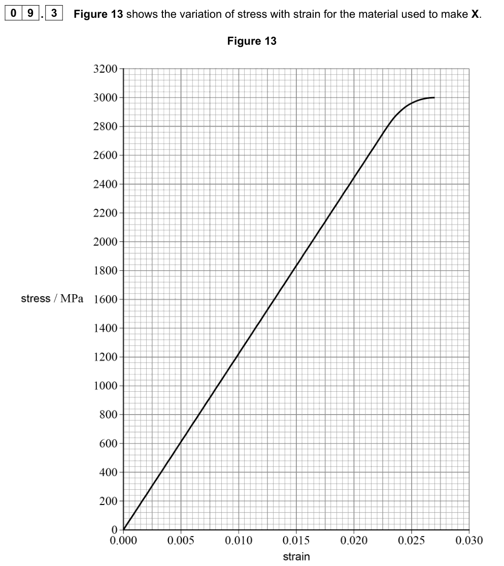
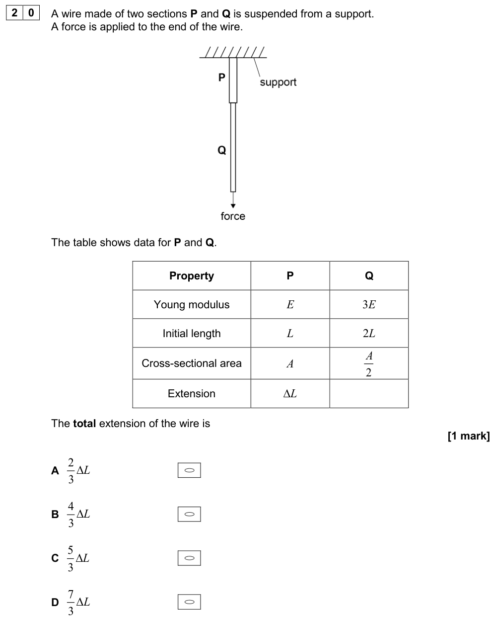
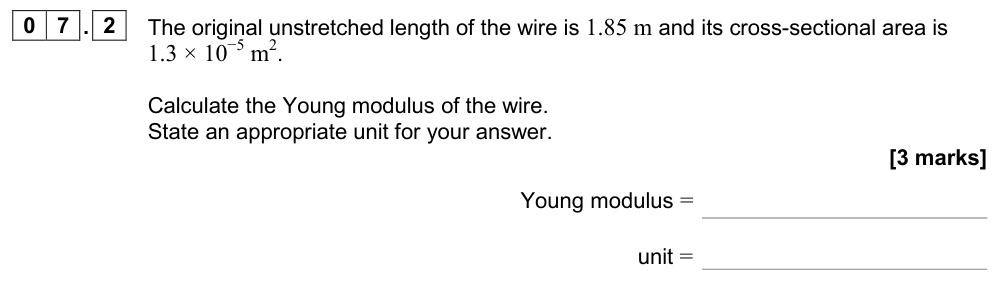
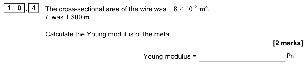
$$E = \frac{\text{tensile stress}}{\text{tensile strain}} = \frac{F/A}{\Delta L/L} = \frac{FL}{A\Delta L}$$
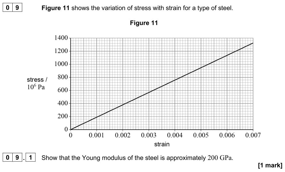
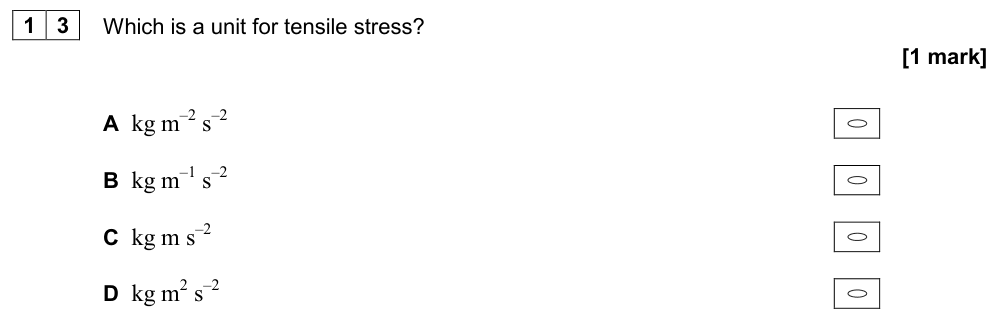
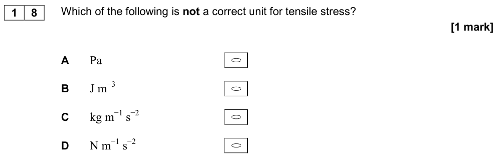
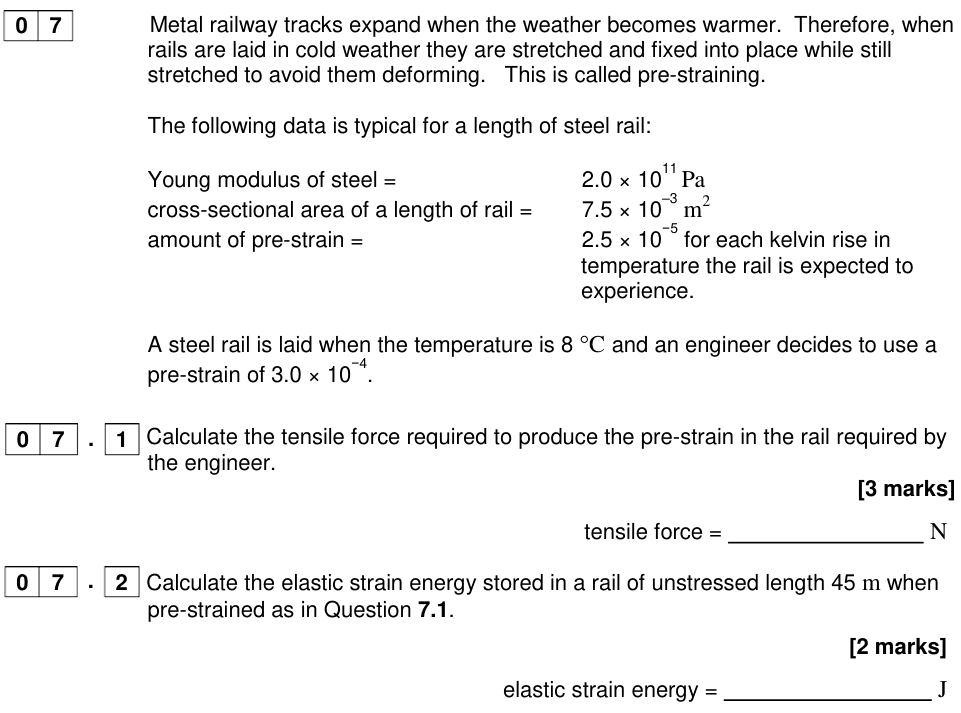
Unit: pascal (Pa), the same as stress, because strain has no unit. Typical values are large, e.g. steel $2.0 \times 10^{11}\ \text{Pa}$ (200 GPa).
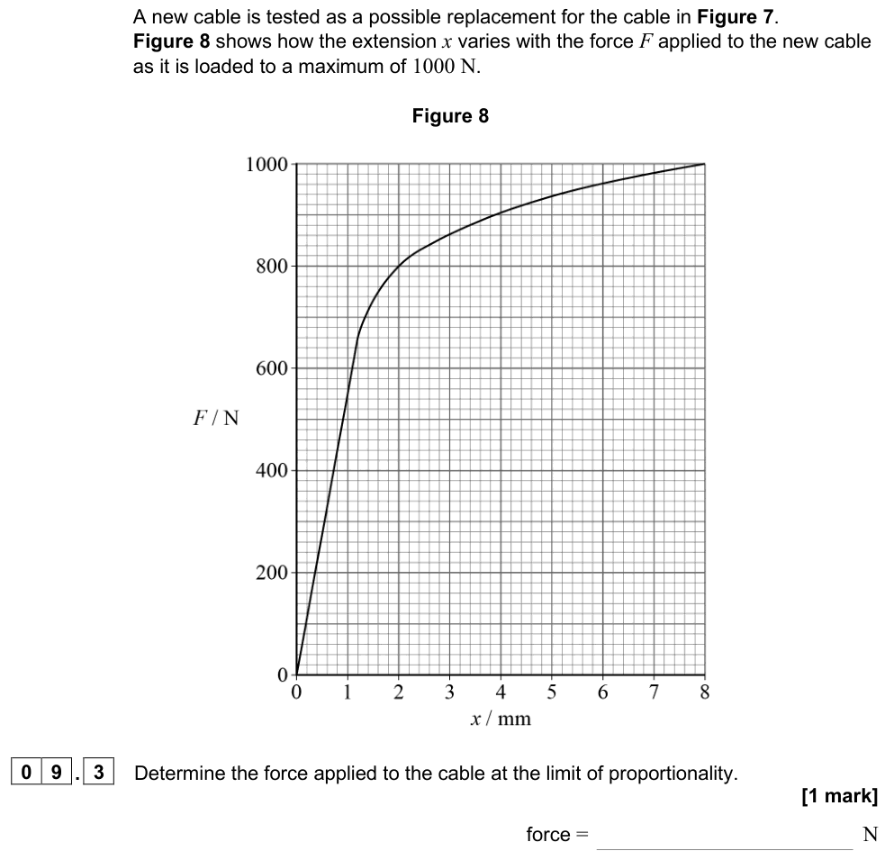
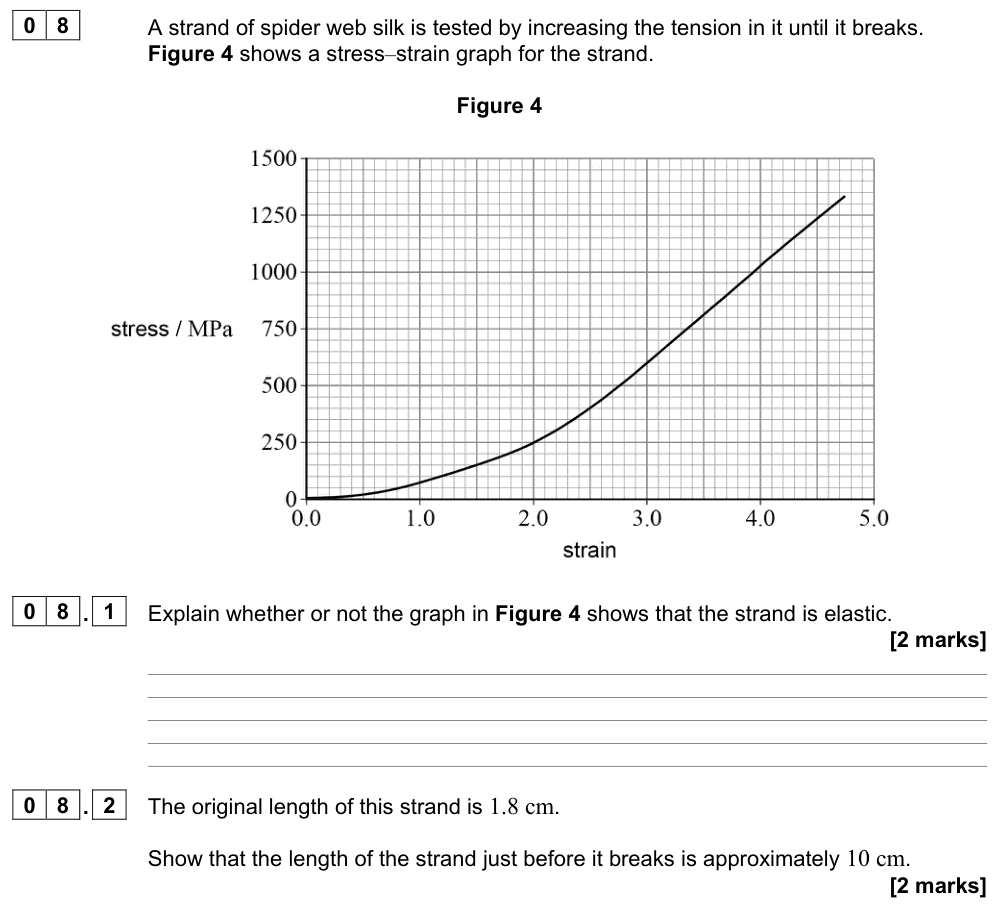
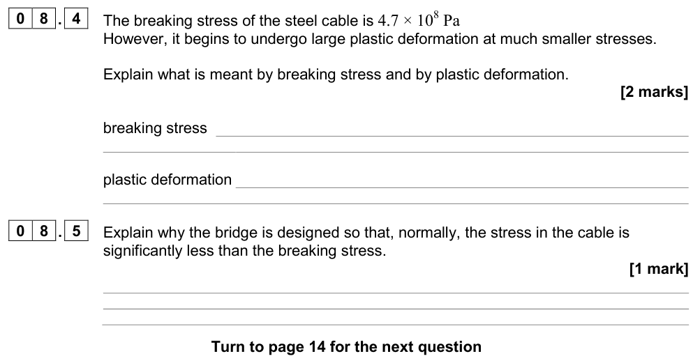
The Young modulus applies only in the region where stress is proportional to strain (up to the limit of proportionality).
| Material | Young modulus / GPa |
|---|---|
| rubber | ~0.01–0.1 |
| nylon | 2–4 |
| bone | ~15 |
| glass | ~70 |
| aluminium | 70 |
| copper | 120 |
| steel | 200 |
| diamond | 1000 |
Worked example: steel cable
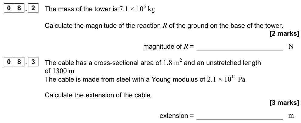
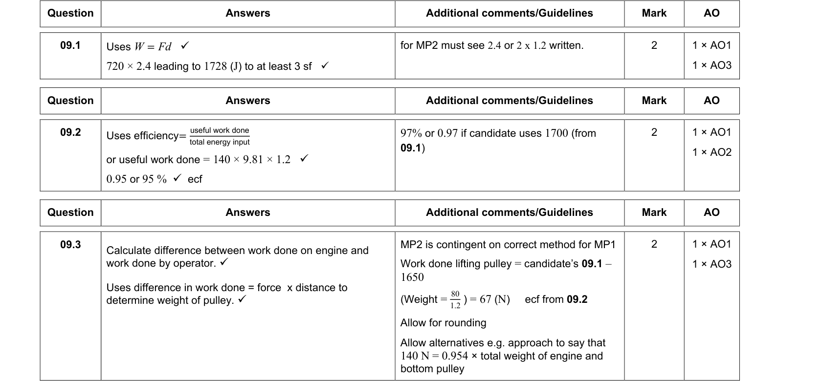
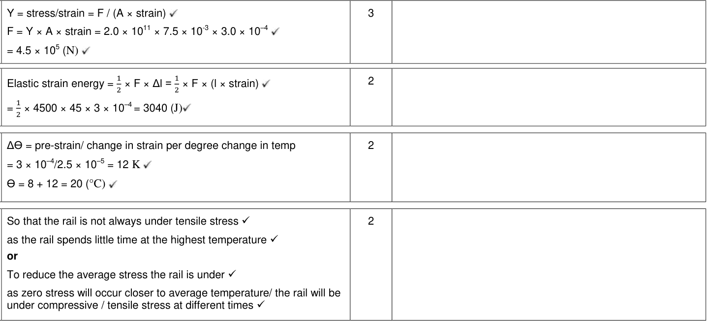
A steel cable 25 m long with cross-sectional area $2.0 \times 10^{-4}\ \text{m}^2$ supports a load of $1.2 \times 10^{4}$ N. $E = 2.0 \times 10^{11}\ \text{Pa}$. Find the extension.
$$\Delta L = \frac{FL}{AE} = \frac{1.2 \times 10^{4} \times 25}{2.0 \times 10^{-4} \times 2.0 \times 10^{11}} = 7.5 \times 10^{-3}\ \text{m} = 7.5\ \text{mm}$$
Exam tip: how extension depends on the wire
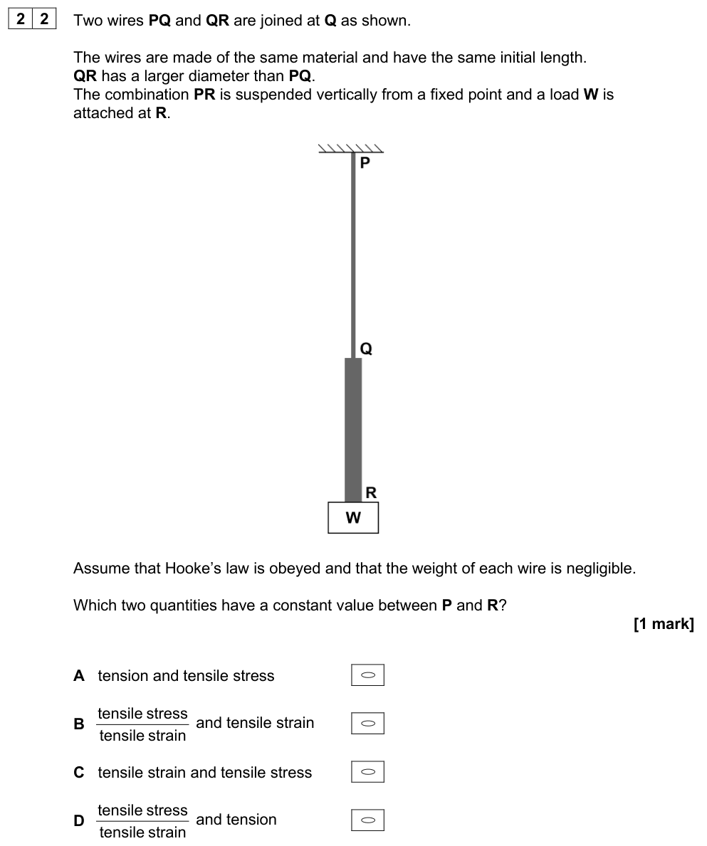
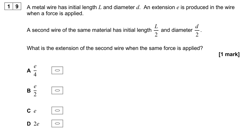
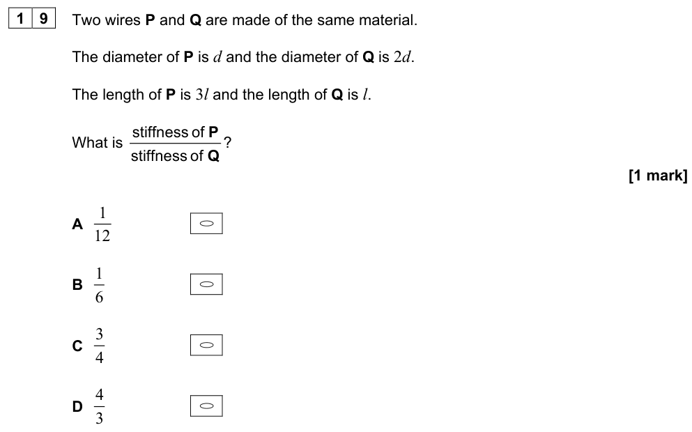
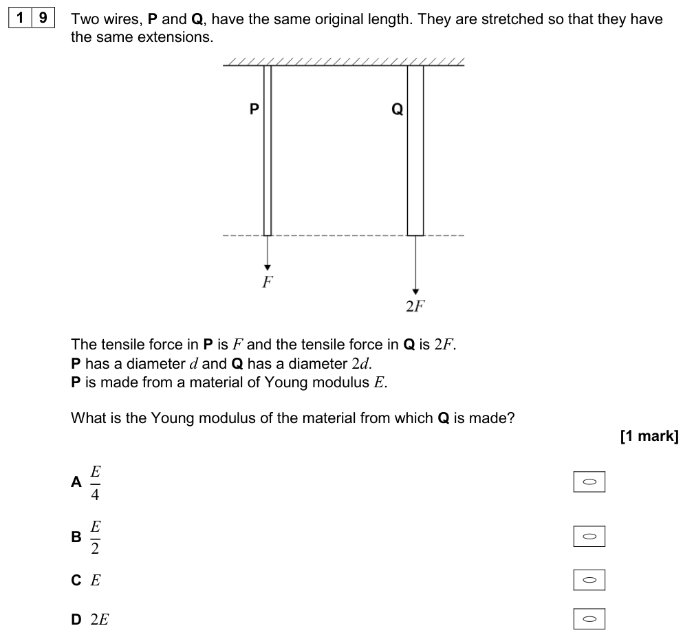
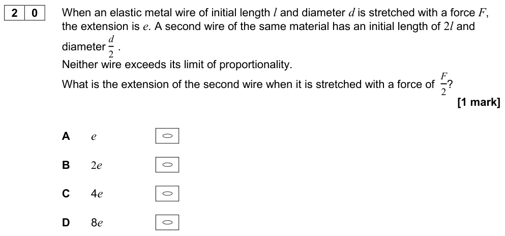
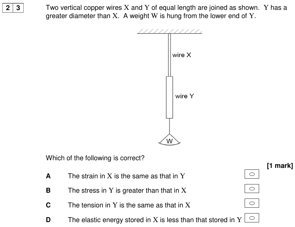
From $\Delta L = \dfrac{FL}{AE}$: extension is proportional to length and inversely proportional to area ($\propto 1/d^2$). A wire of the same material with twice the diameter stretches one quarter as much. A wire that is twice as long stretches twice as much.
Stress–strain graphs
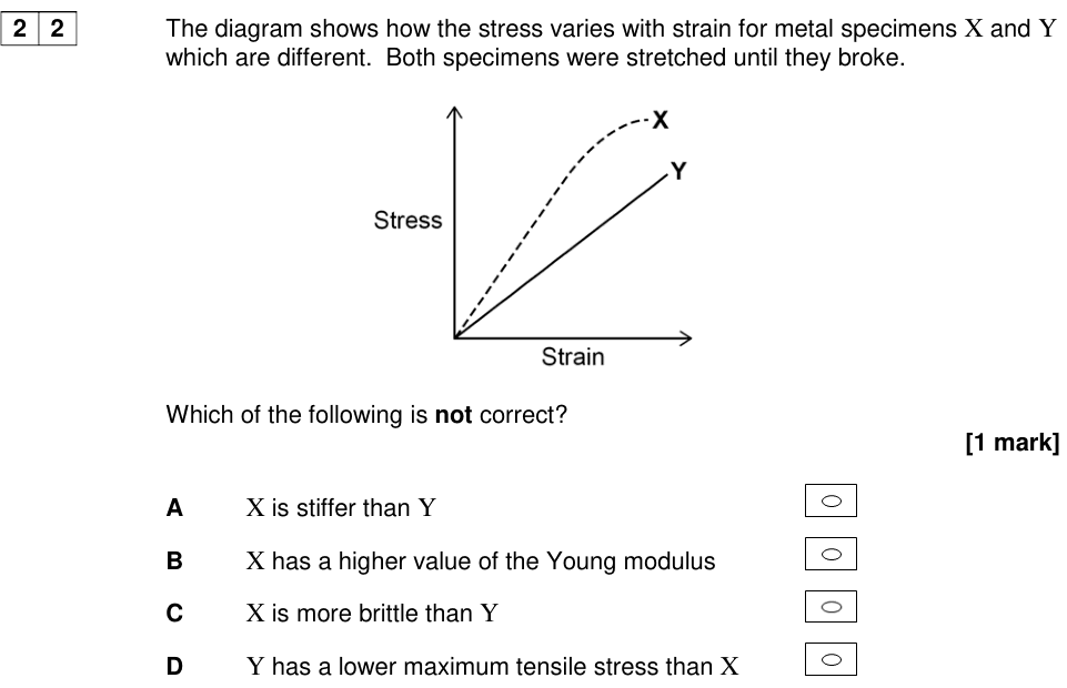
Reading a stress–strain graph
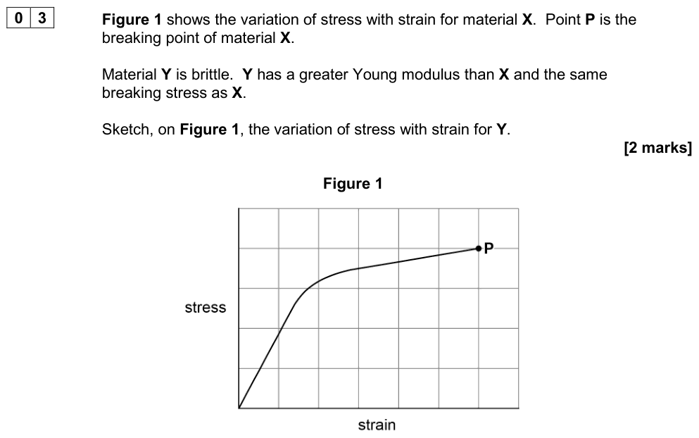
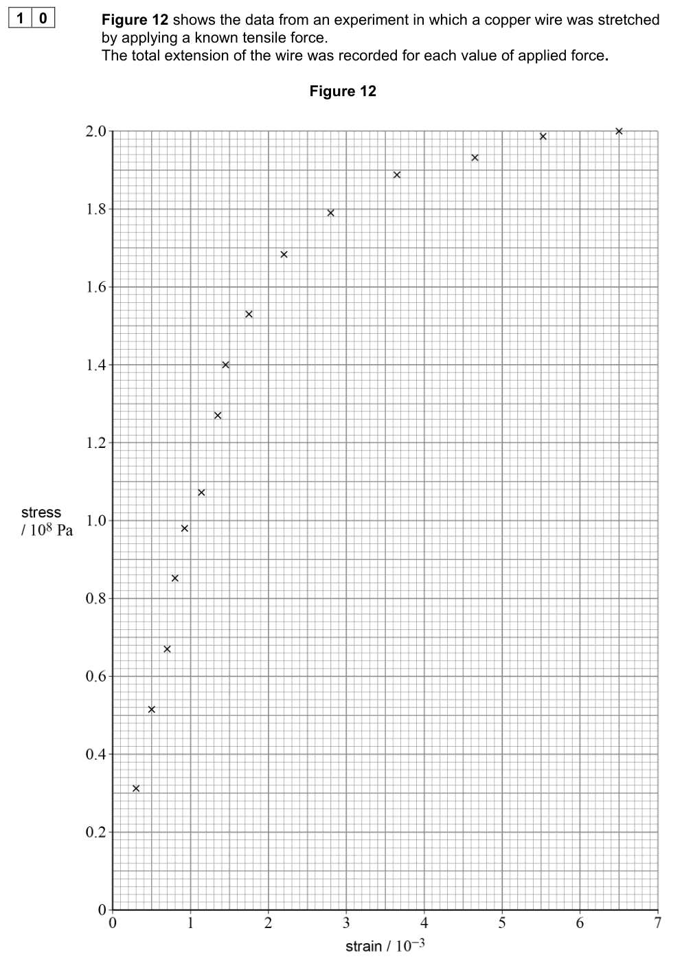
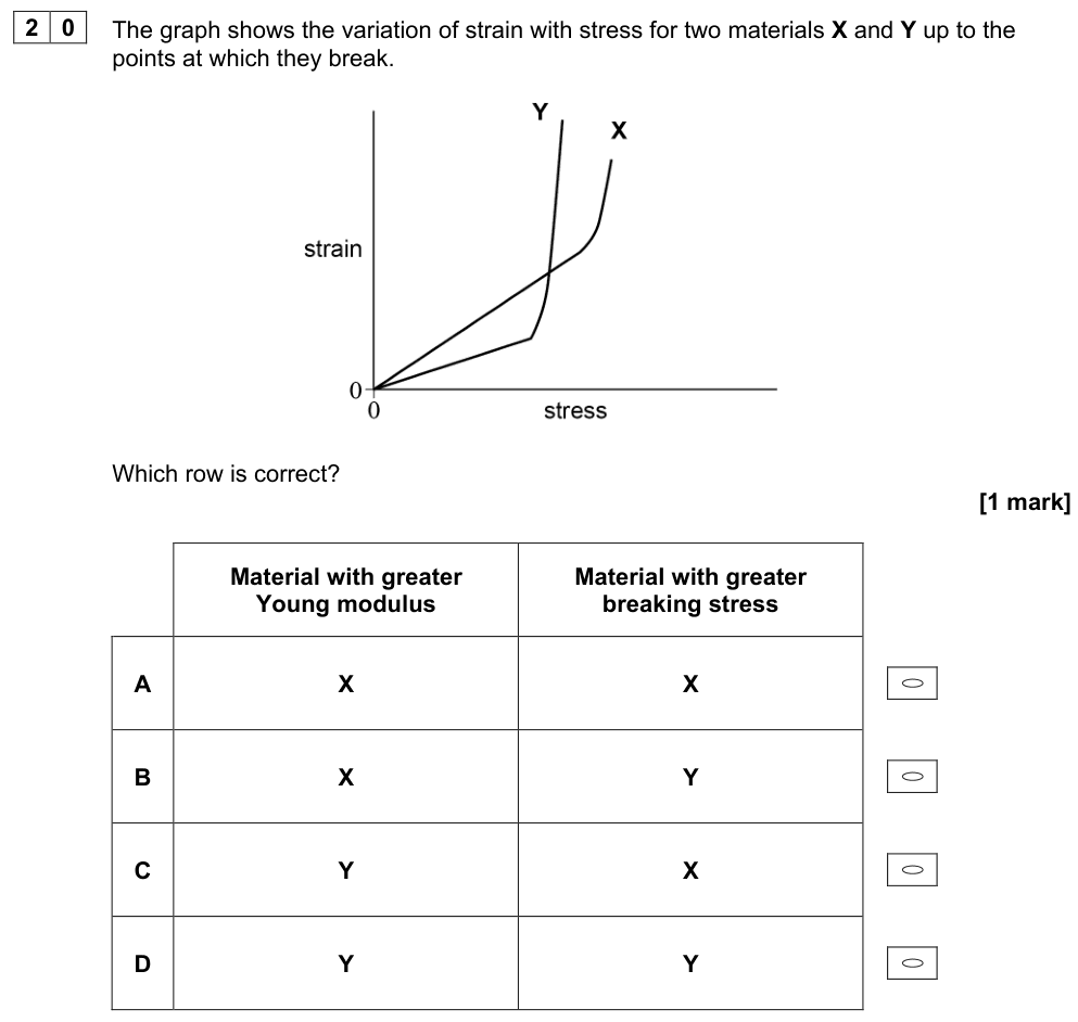
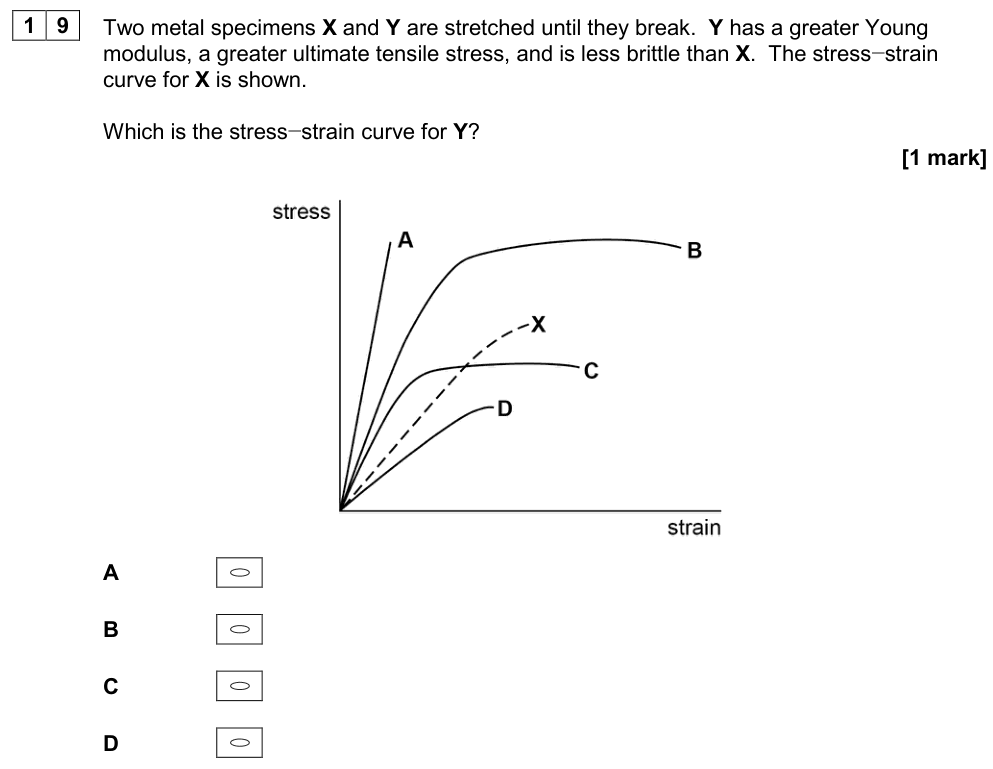
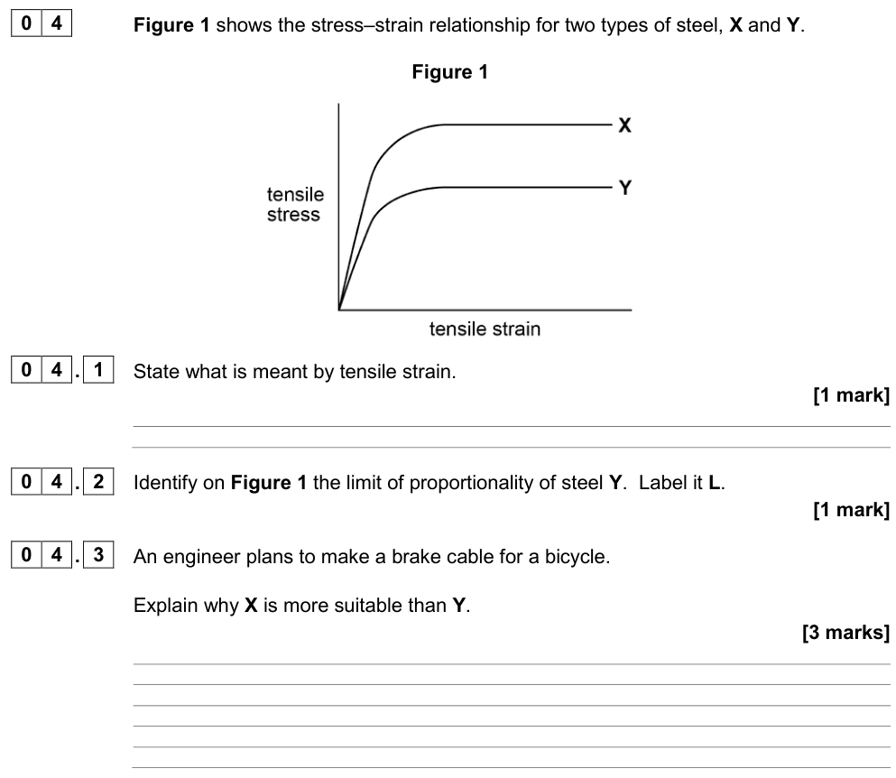
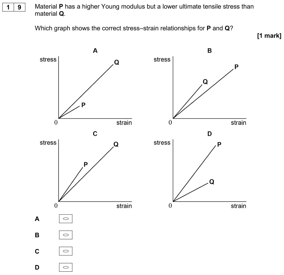
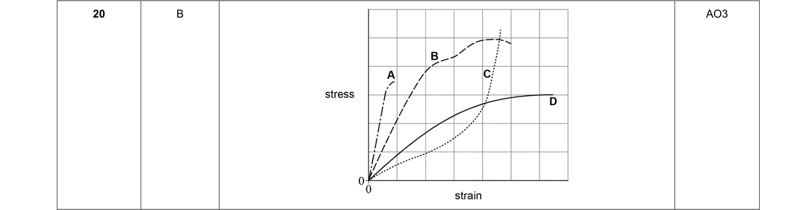
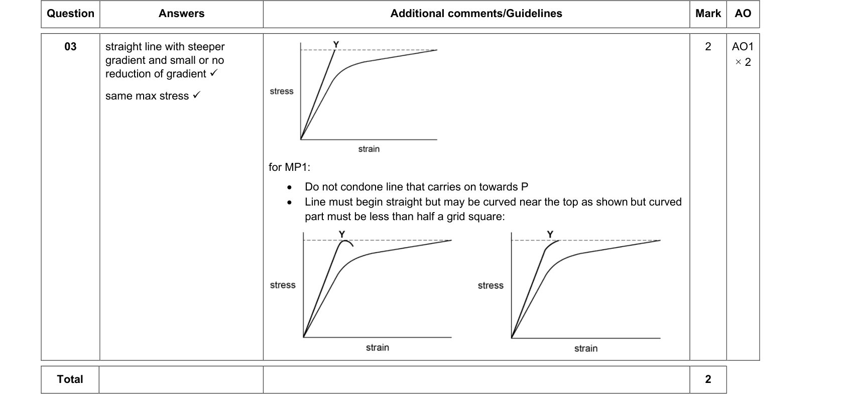
- Gradient of the straight-line section = Young modulus $E$ (stiffness).
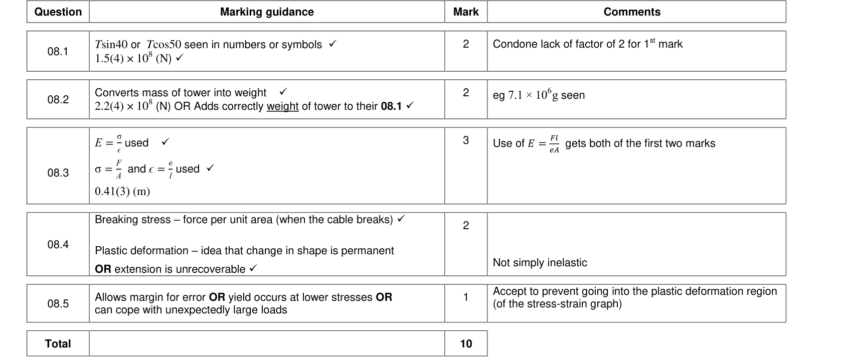
- Highest point = ultimate tensile stress (breaking stress): the strength.
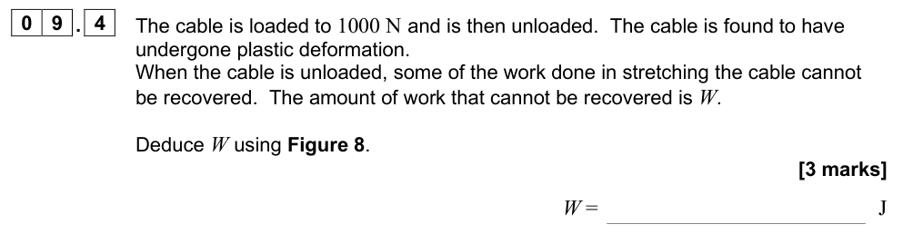
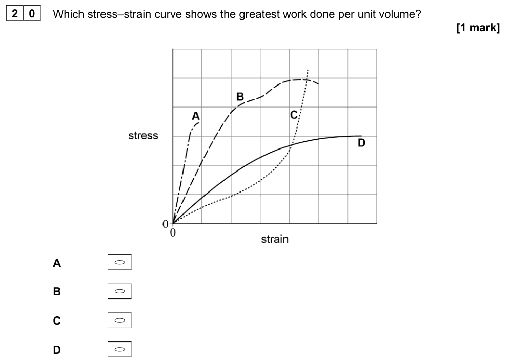
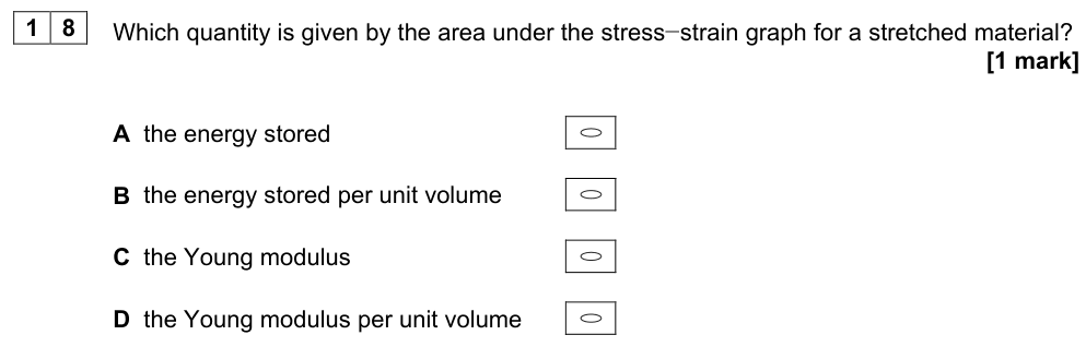
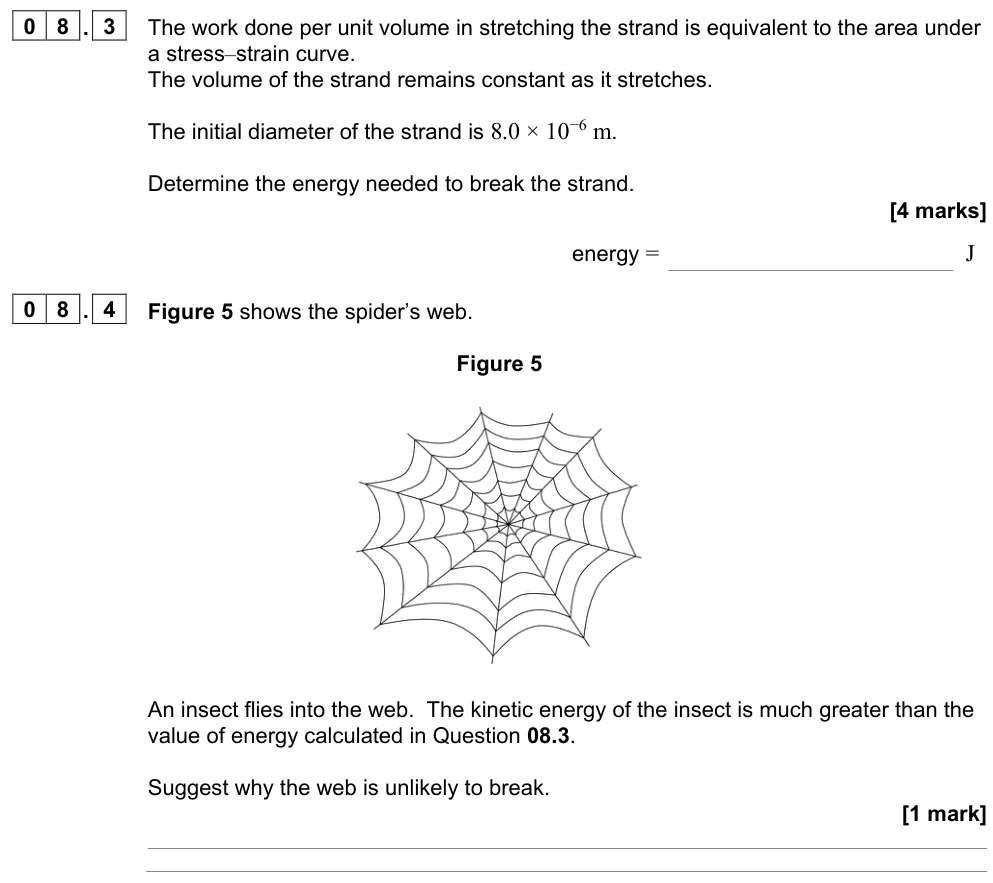
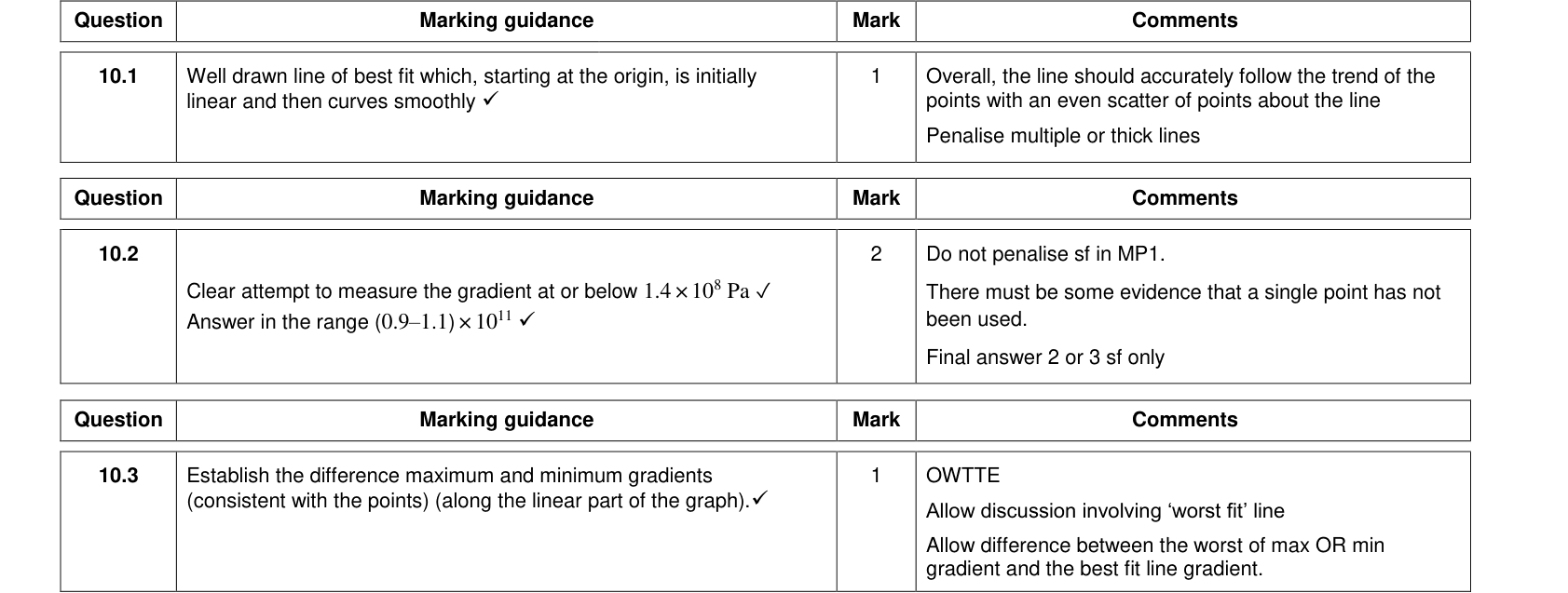
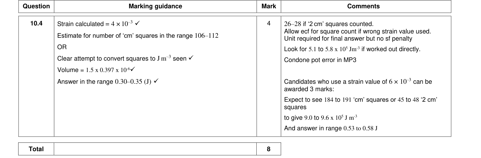
- Area under the graph = energy stored per unit volume (strain energy density). For the linear region this is $\tfrac12 \sigma\varepsilon$ in J m⁻³.
- Large strain after the elastic limit = ductile; breaks at the end of the straight section = brittle.
Comparing materials
| Property | What it means | On the graph |
|---|---|---|
| Stiff | high Young modulus | steep initial gradient |
| Strong | high breaking stress | high maximum stress |
| Ductile | large plastic deformation before breaking | long curved region |
| Brittle | little or no plastic deformation | breaks at the end of the straight line |
| Tough | absorbs a lot of energy before breaking | large area under the graph |
Required practical 2: the Young modulus of a wire
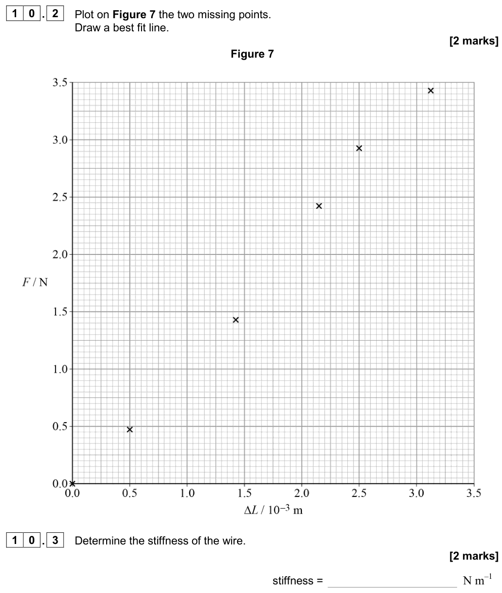
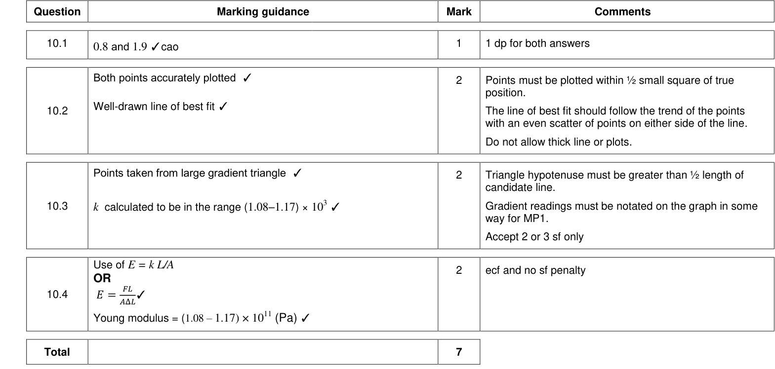
Required practical 2: load–extension graph for a wire and the Young modulus
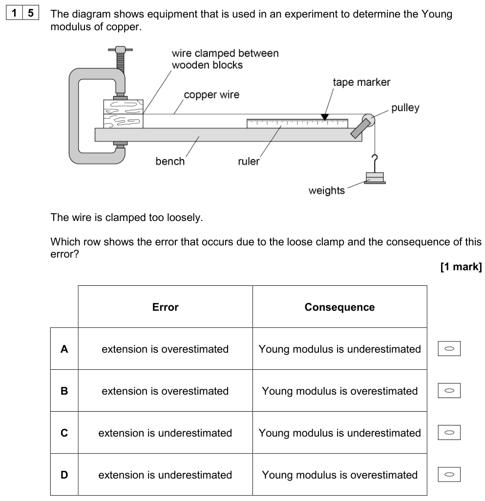
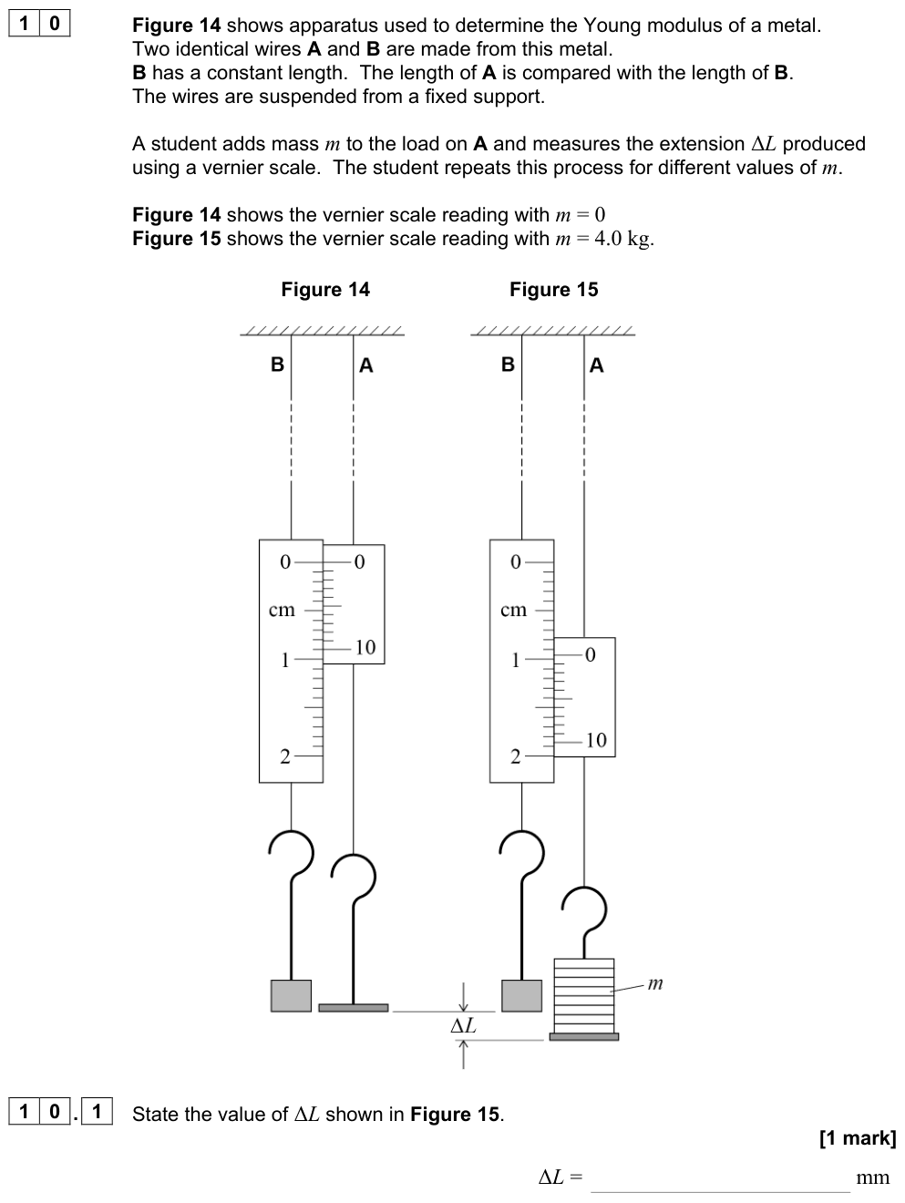
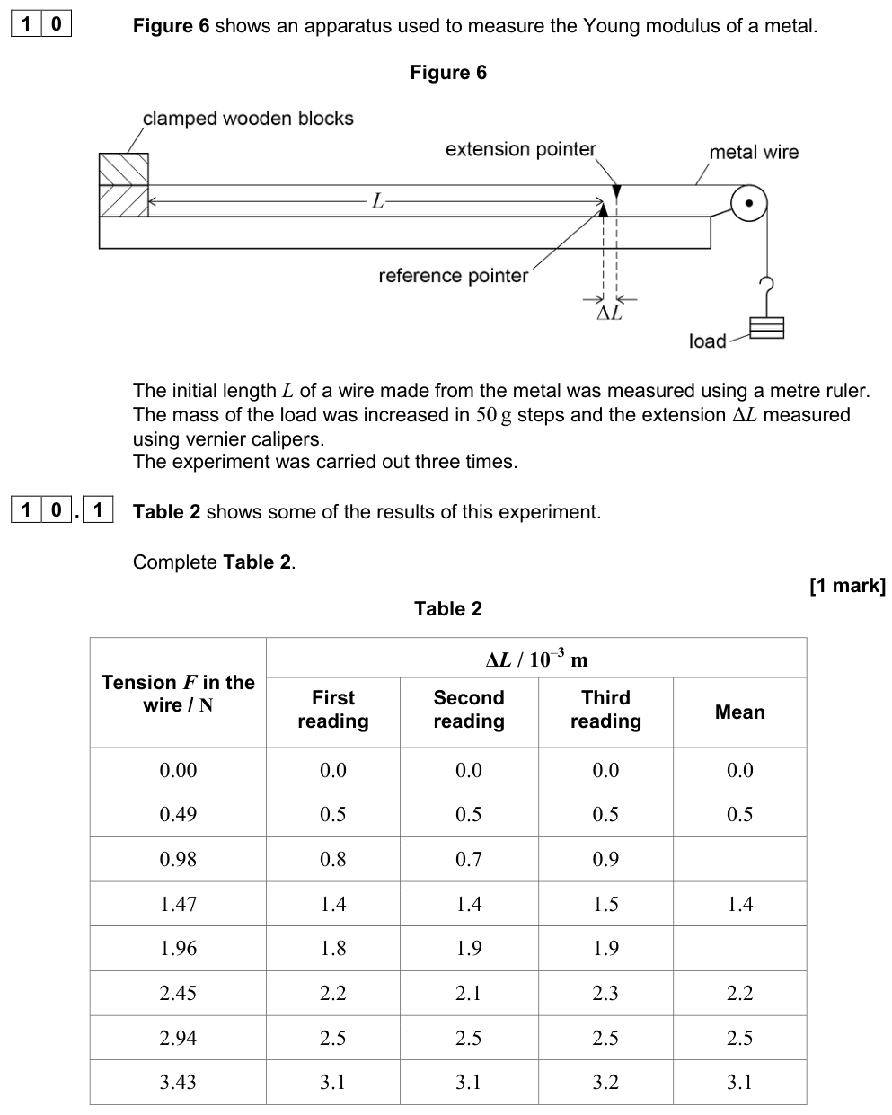
Apparatus. A long thin wire (2–3 m) is clamped at one end and passes over a pulley to a mass hanger, or it hangs vertically beside an identical reference wire. A marker on the wire moves along a millimetre scale, or a vernier scale compares the test wire with the reference wire.
Method.
- Measure the original length $L$ from the clamp to the marker with a metre rule or tape.
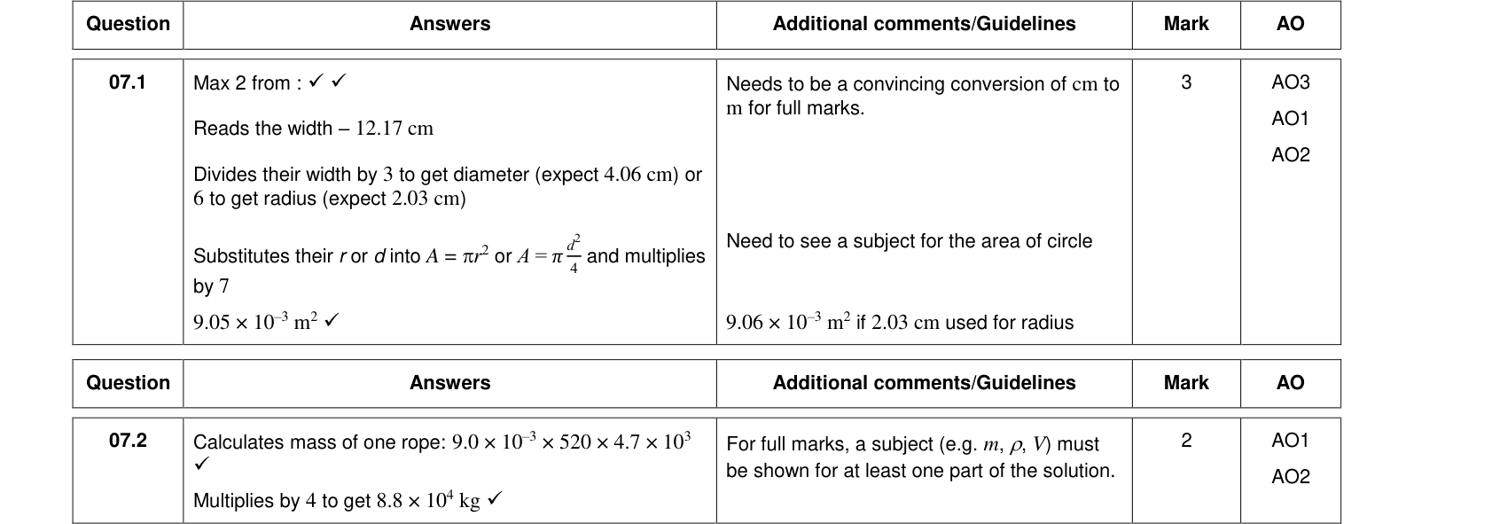
- Measure the diameter $d$ with a micrometer at several places along the wire and in different orientations. Calculate the mean, then $A = \pi d^2/4$.
- Add a small initial load to straighten the wire, and take that reading as zero extension.
- Add masses in equal steps, recording the extension each time. Check the extension returns to zero when the load is removed, to confirm you have not passed the elastic limit.
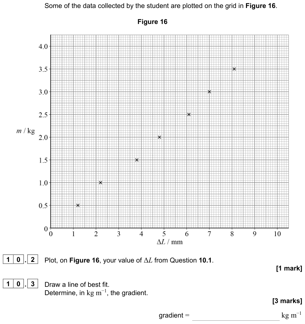
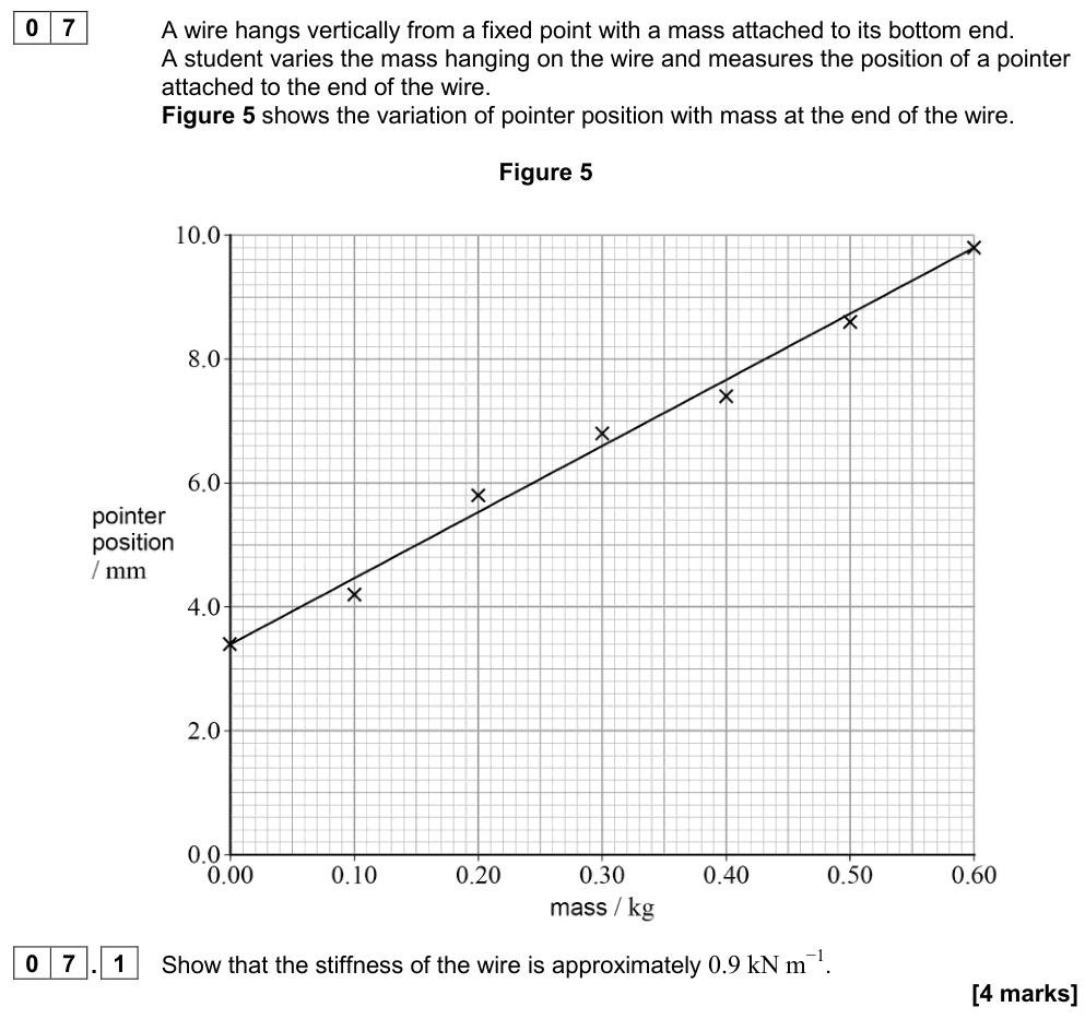
Analysis. Plot a graph of load $F$ (y-axis) against extension $\Delta L$ (x-axis). In the straight-line region:
$$\text{gradient} = \frac{F}{\Delta L} \quad \Rightarrow \quad E = \text{gradient} \times \frac{L}{A}$$
Improving accuracy.
- The reference wire (or comparison wire) compensates for temperature changes and sagging of the support, which would otherwise appear as extension.
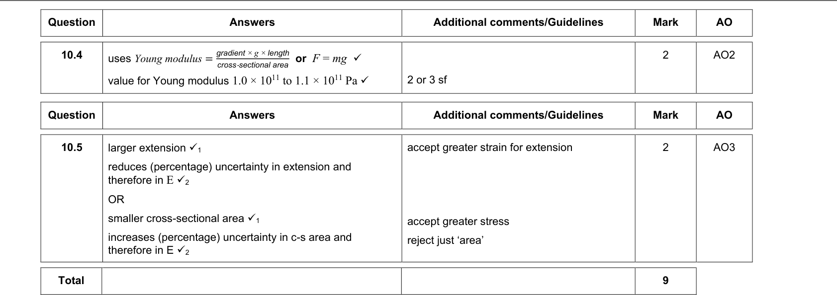
- Using a long, thin wire makes the extension large enough to measure with a small percentage uncertainty.
- The diameter has the largest percentage uncertainty and it is squared, so measure it carefully with a micrometer at several points.
- Safety: wear eye protection in case the wire snaps, and put a box or padding under the masses.
Worked example: analysing results
A wire of length 2.50 m and diameter 0.38 mm gives a load–extension gradient of $1.15 \times 10^{4}\ \text{N m}^{-1}$.
$A = \pi(0.38 \times 10^{-3})^2/4 = 1.13 \times 10^{-7}\ \text{m}^2$.
$E = 1.15 \times 10^{4} \times \dfrac{2.50}{1.13 \times 10^{-7}} = 2.5 \times 10^{11}\ \text{Pa}$.
Summary
- $E = \dfrac{\text{stress}}{\text{strain}} = \dfrac{FL}{A\Delta L}$, measured in Pa; a property of the material.
- On a stress–strain graph: gradient = $E$; maximum stress = UTS; area = energy per unit volume.
- Required practical 2: plot $F$ against $\Delta L$; $E = \text{gradient} \times L/A$; measure $d$ with a micrometer; use a reference wire.