Errors: random and systematic
No measurement is perfect. The difference between a measured value and the true value is the measurement error. There are two kinds, and they behave very differently.
Random error
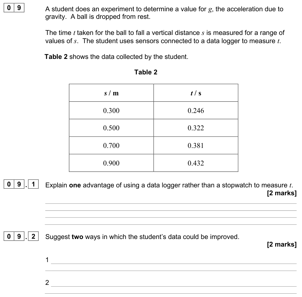
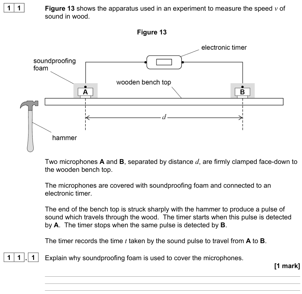
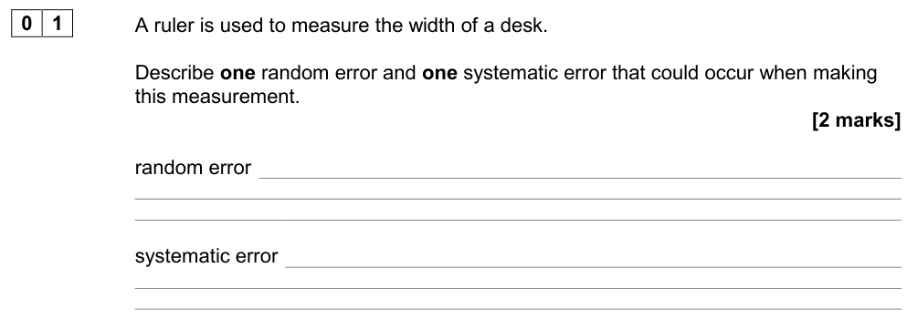
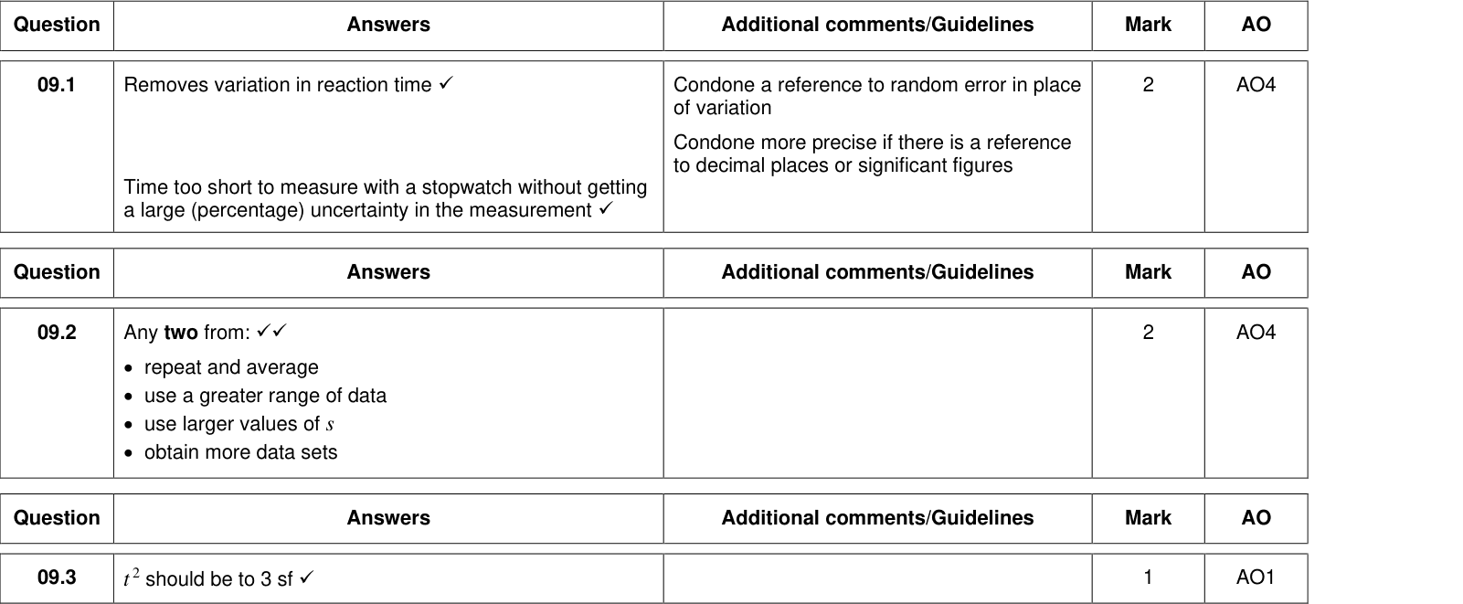
An error that makes readings scatter unpredictably above and below the true value. Examples: judging when a pendulum passes a mark, fluctuations in a reading, slight changes in conditions, human reaction time varying from reading to reading.
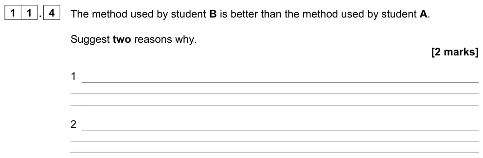
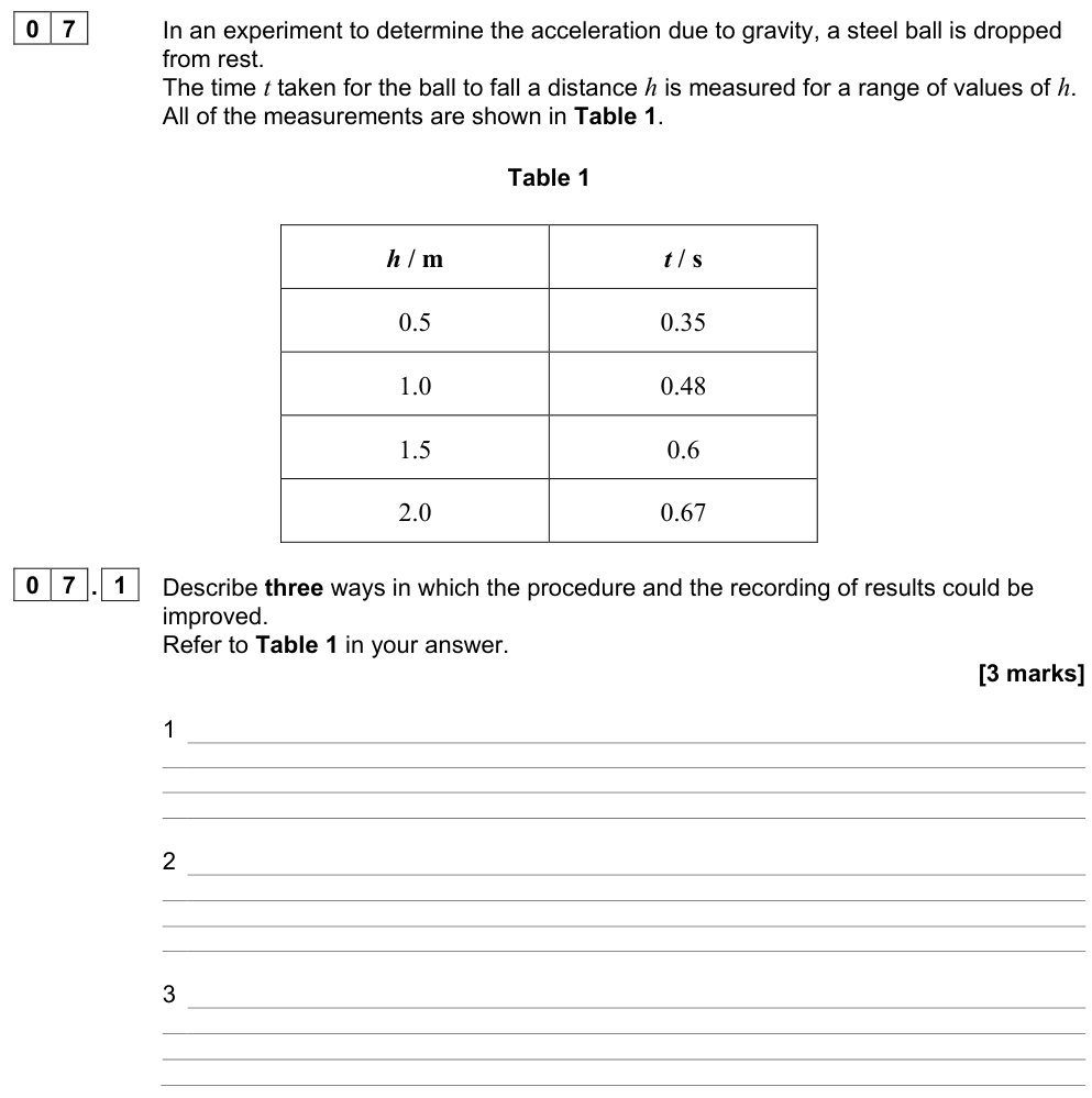
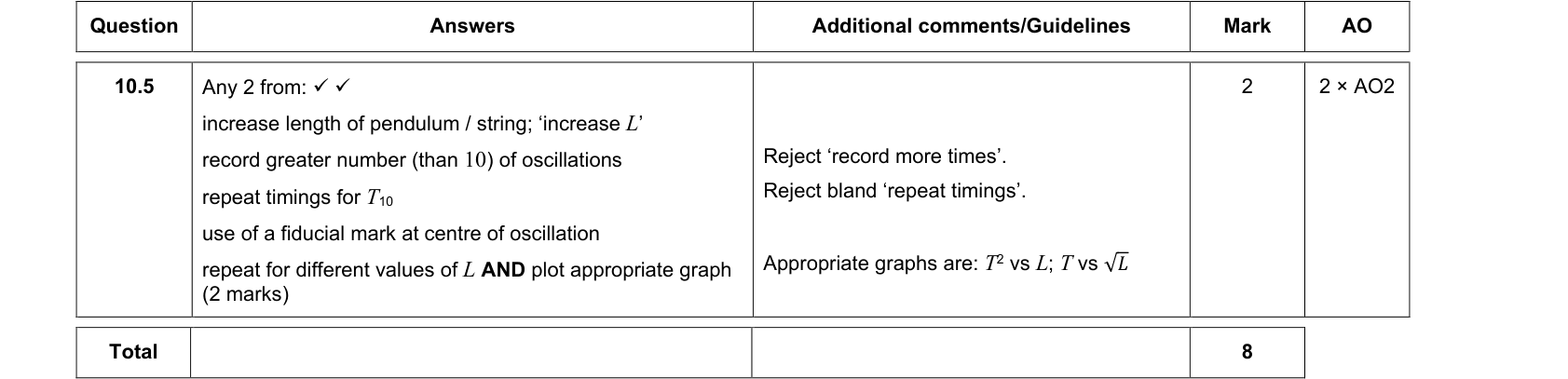
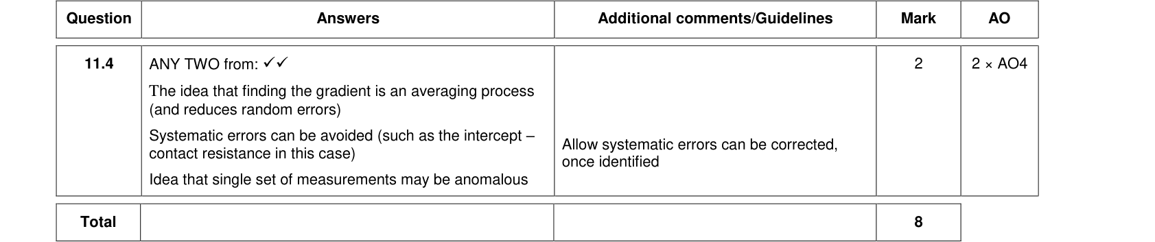
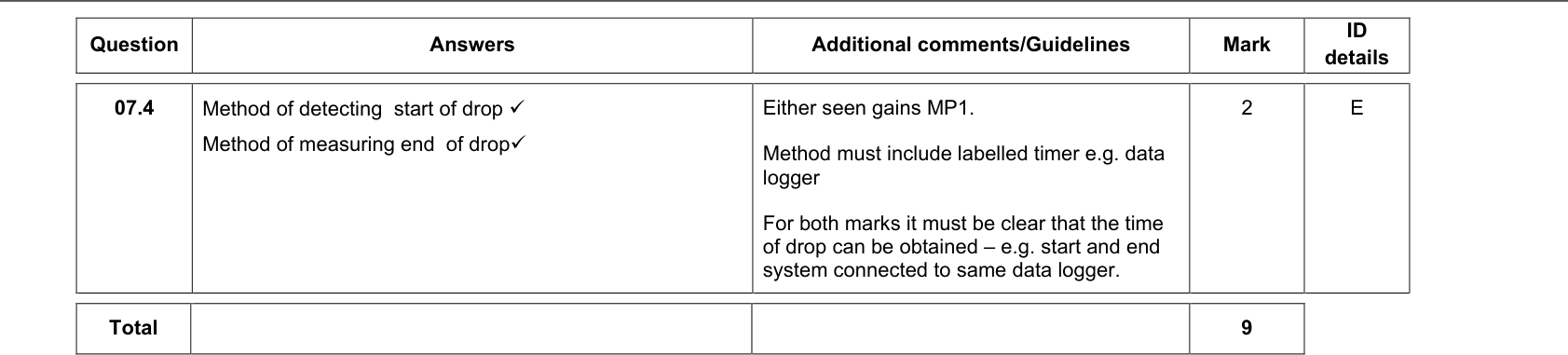
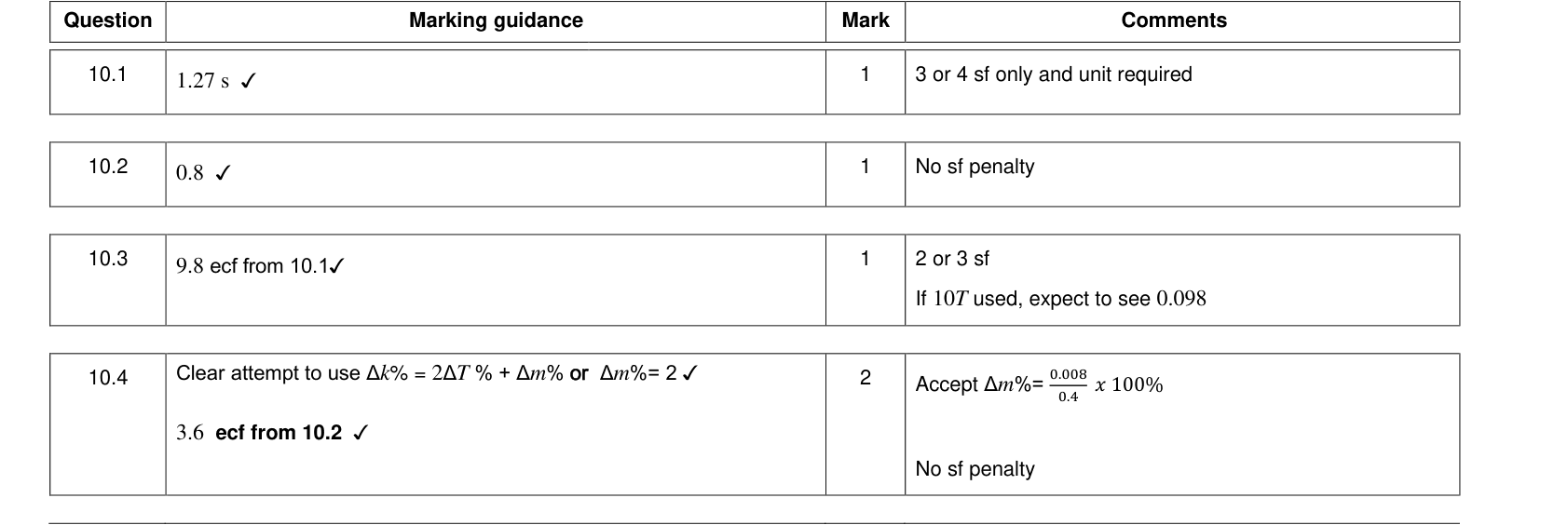
Reduce random errors by repeating readings and calculating a mean, by measuring larger quantities (e.g. time 20 oscillations rather than 1), or by using data-loggers and light gates. Random errors can never be removed completely.
Systematic error
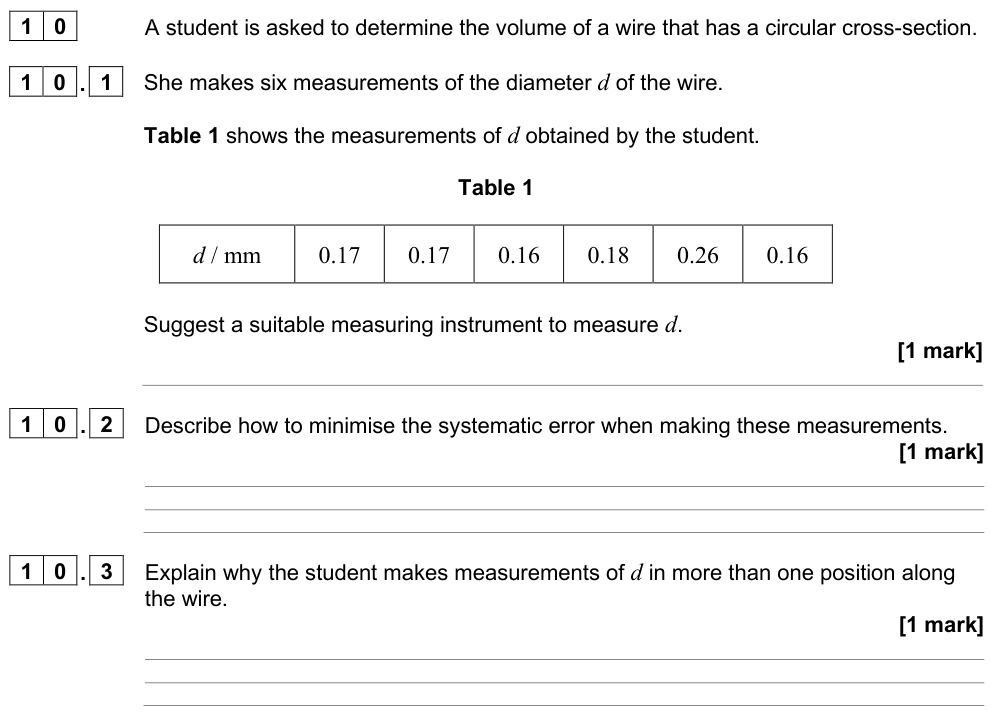
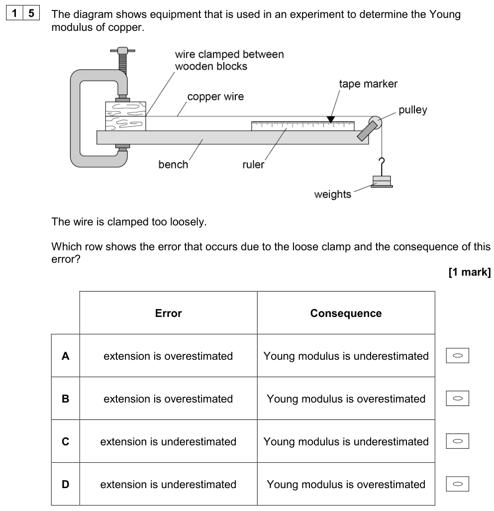
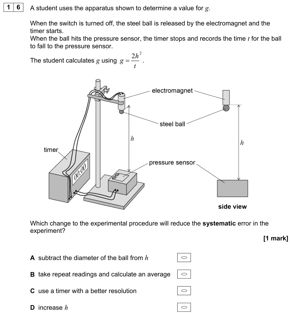
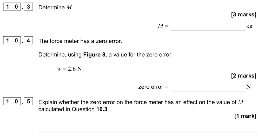
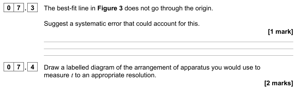
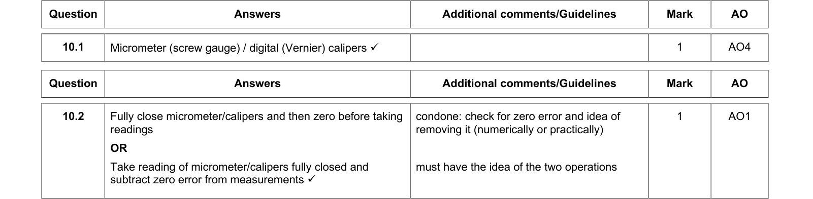
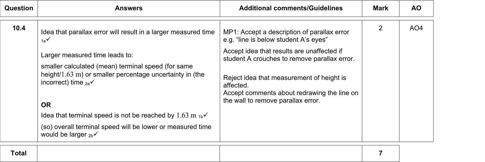
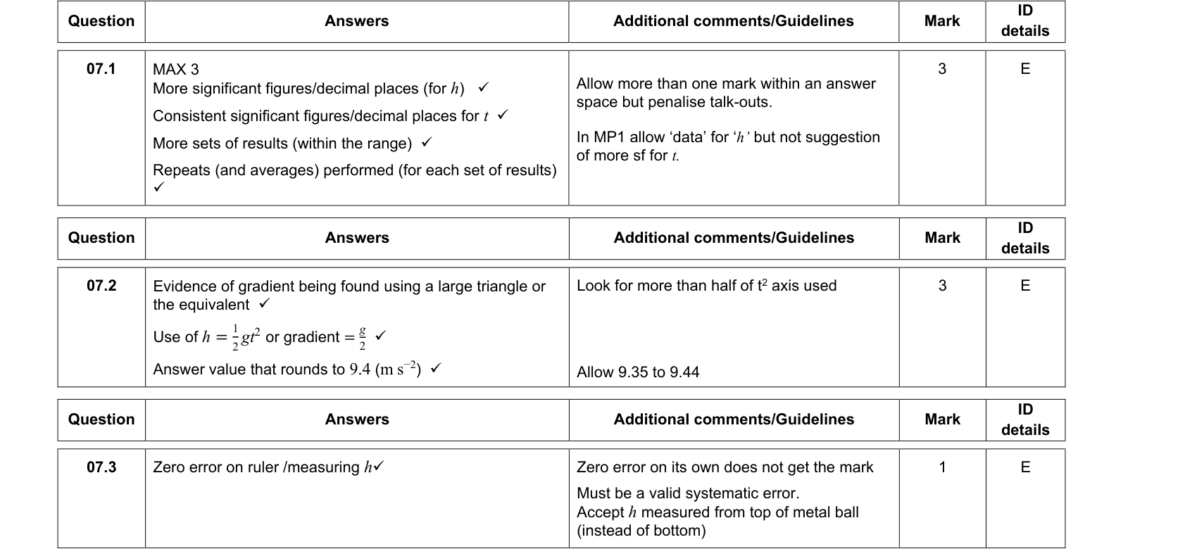
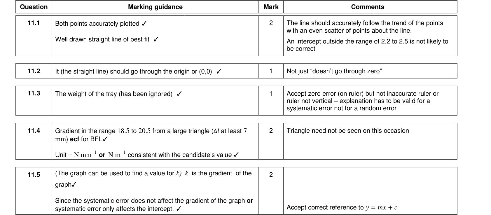
An error that shifts every reading by the same amount or in the same direction. Examples: a zero error on a micrometer or meter, an incorrectly calibrated scale, always reading a scale from the same wrong angle (parallax), a consistent reaction-time delay.
Repeating readings does not reduce a systematic error. Remove it by recalibrating, correcting for the zero error (subtracting it from every reading), or improving the technique (e.g. reading scales at eye level).
Exam tip
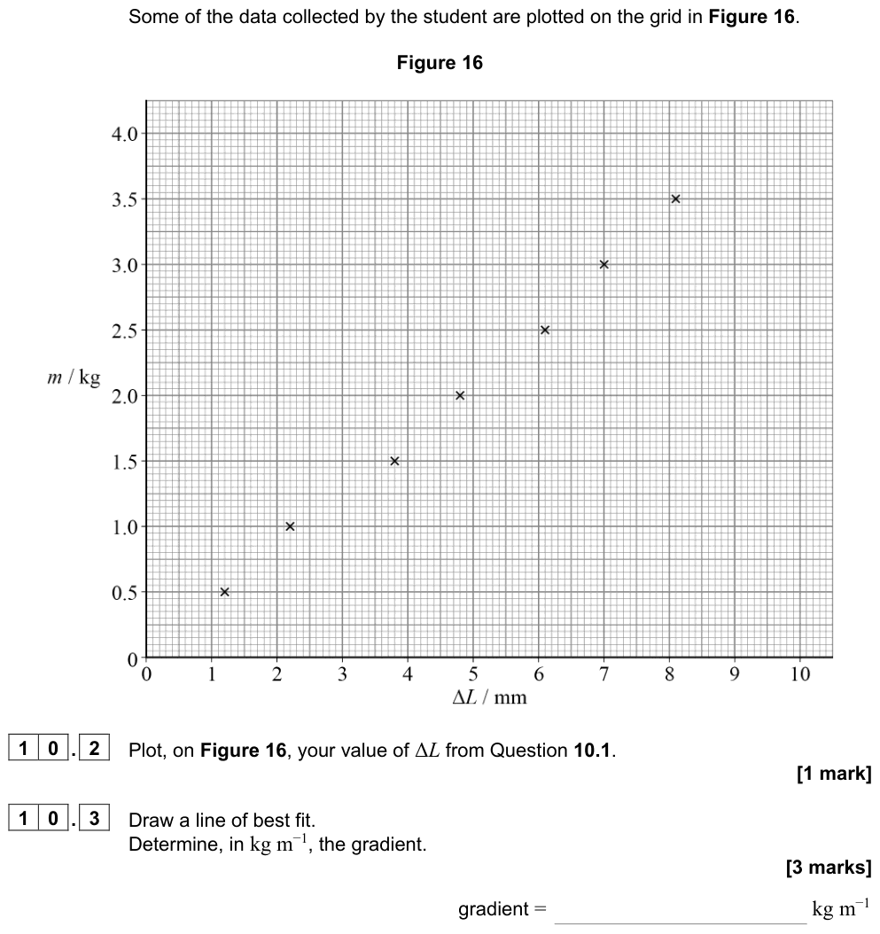
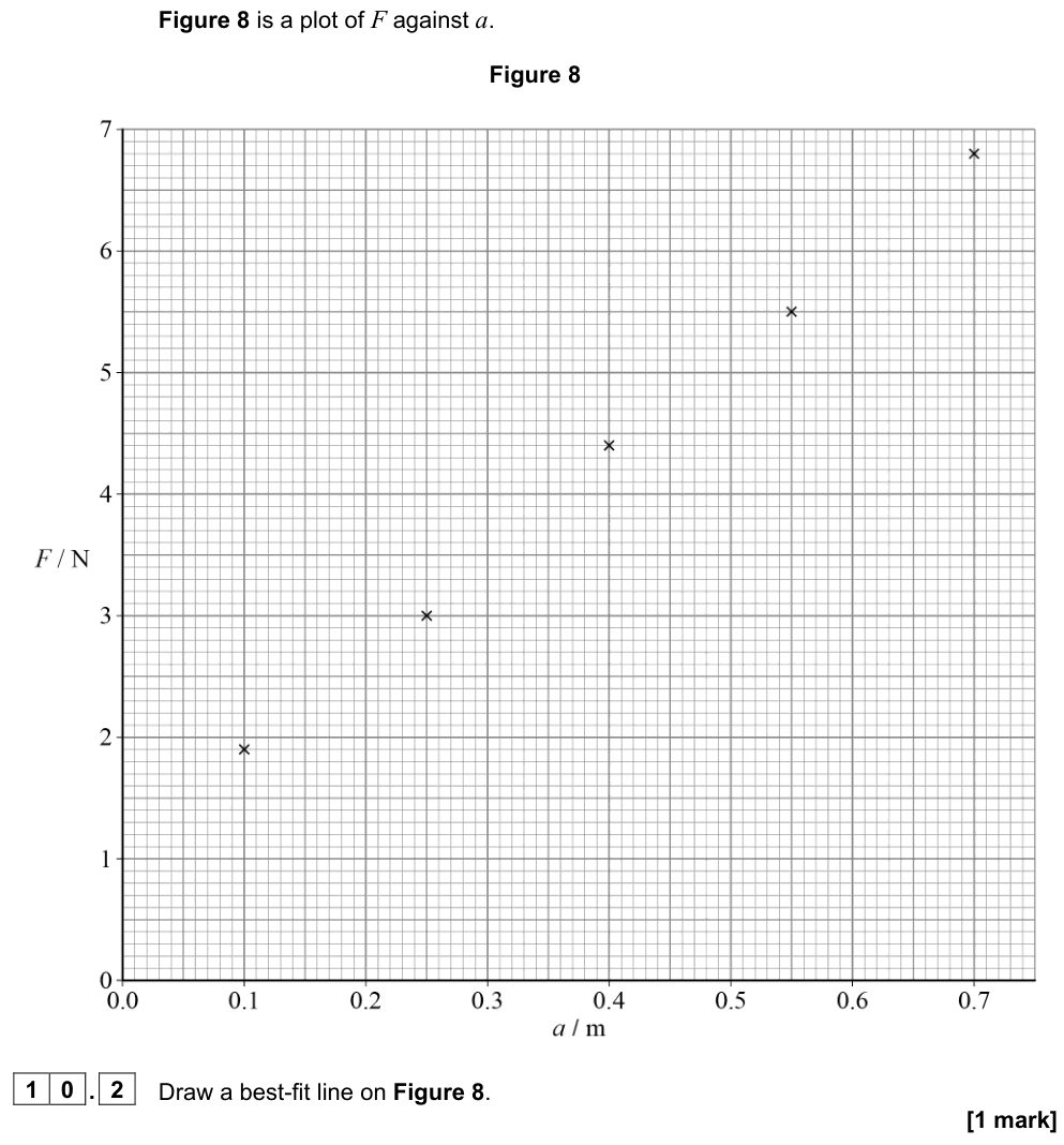
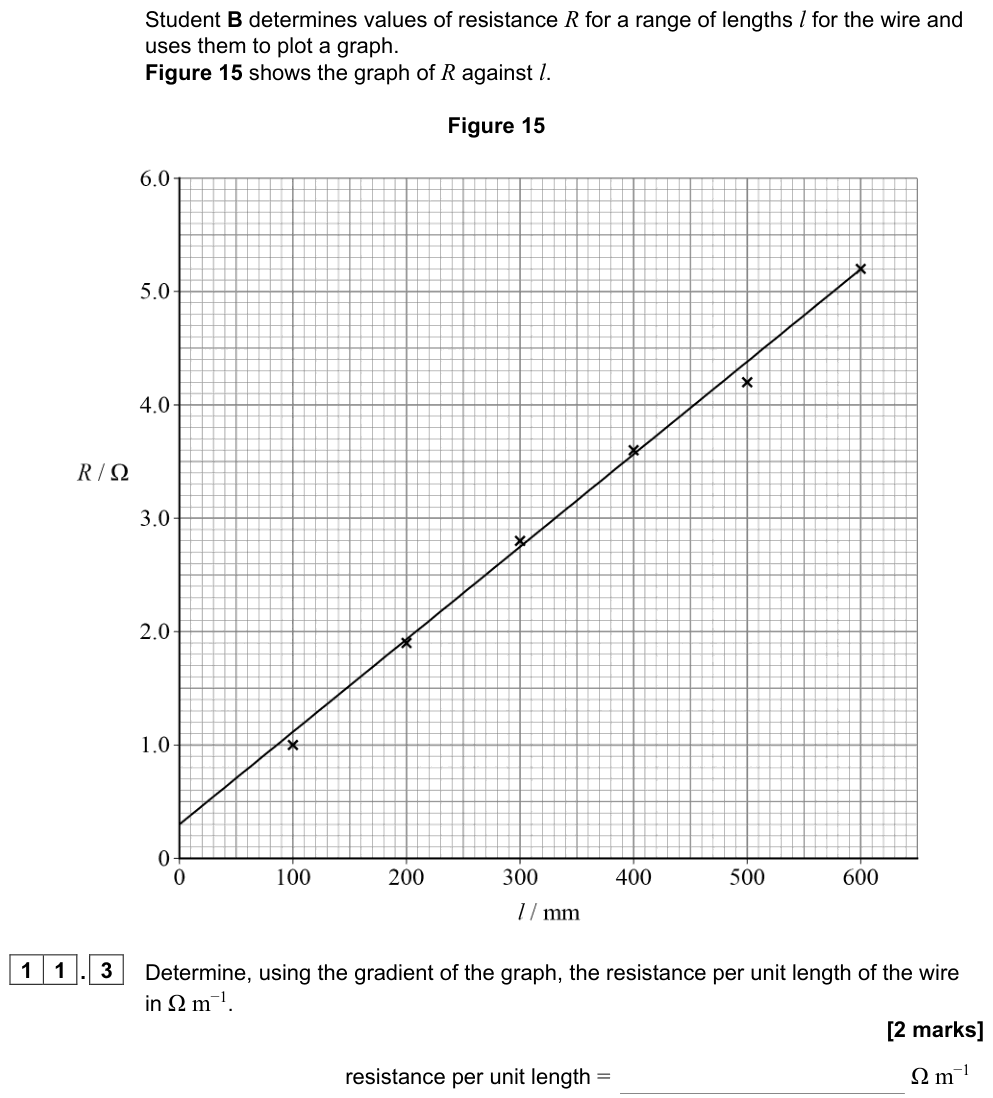
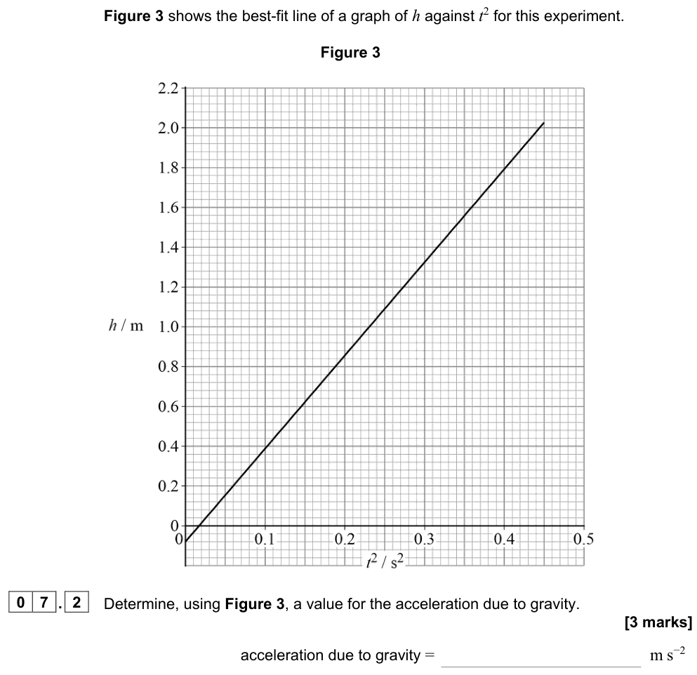
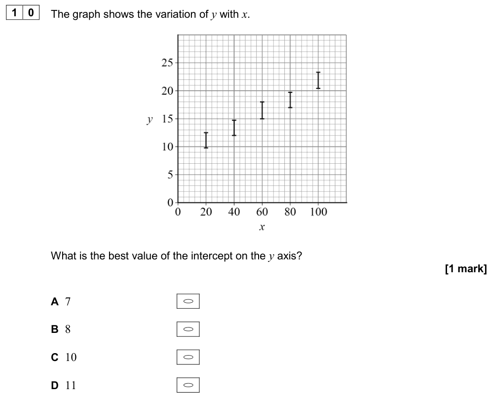
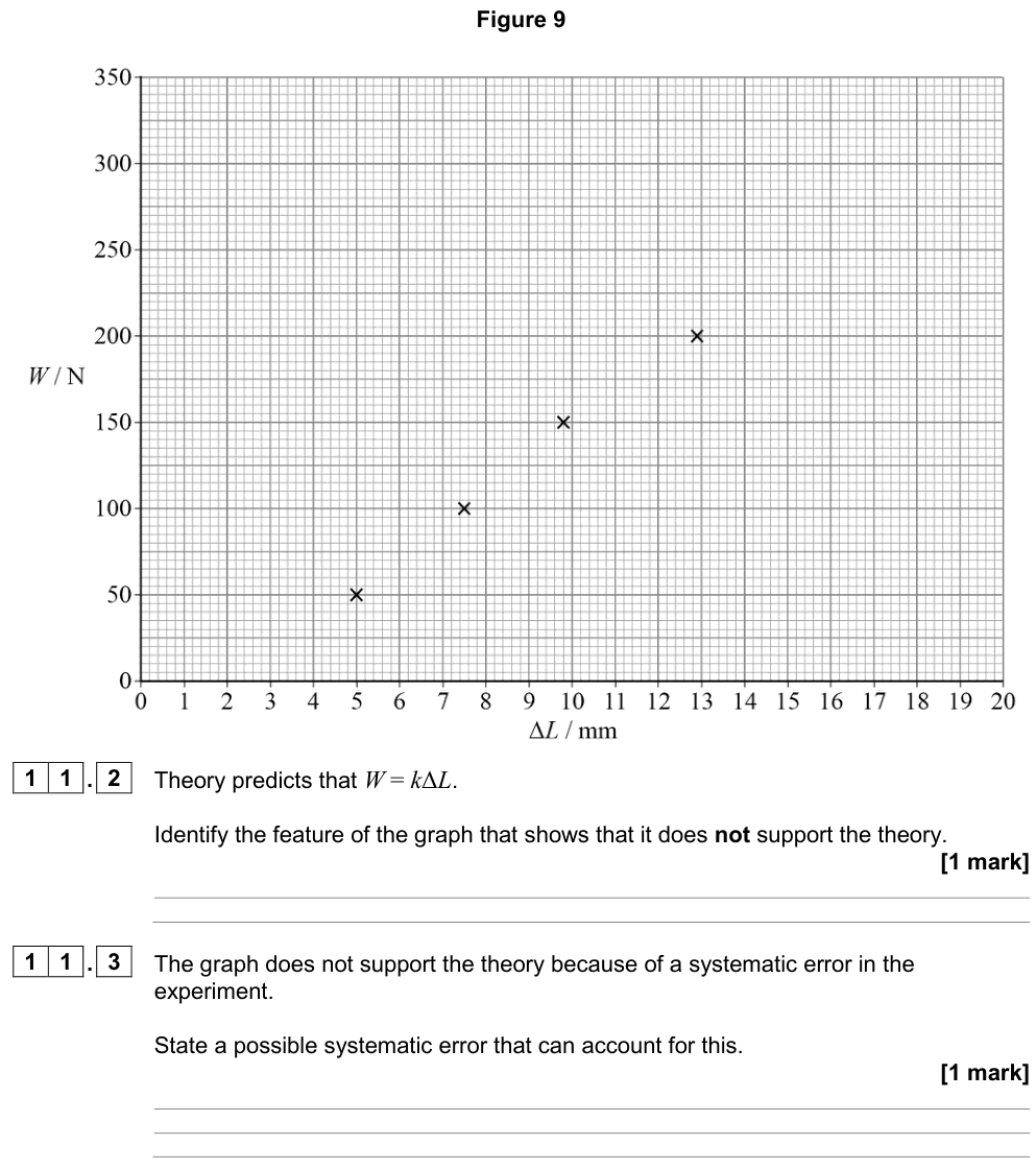
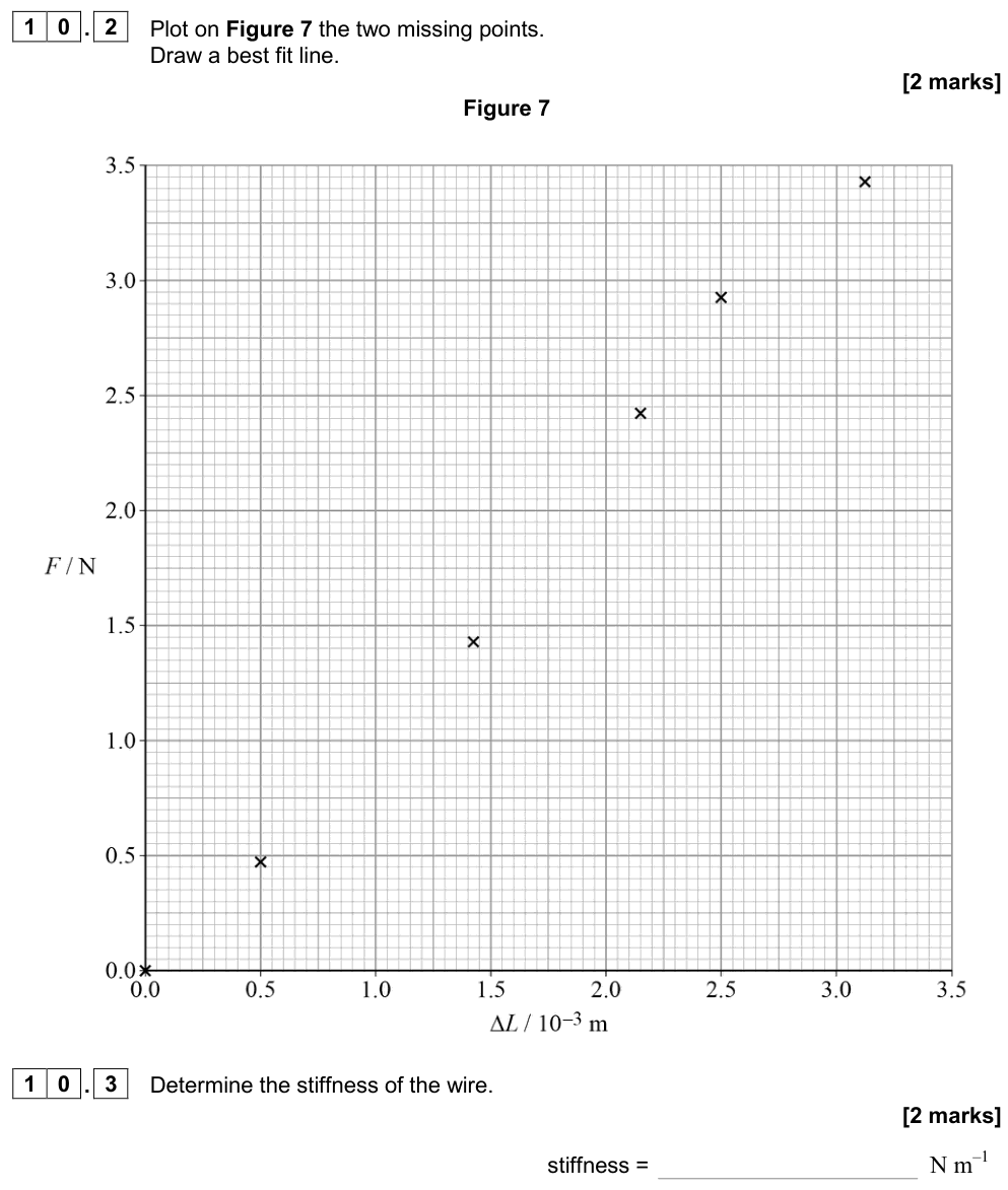
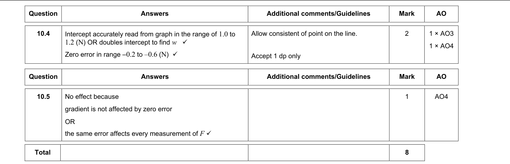
On a graph, a systematic error usually shows up as a line of the correct gradient that does not pass through the origin when it should (a non-zero intercept). Random errors show up as scatter of points about the best-fit line.
Key measurement terms
These definitions come from the AQA practical vocabulary. Learn them word for word.
| Term | Meaning |
|---|---|
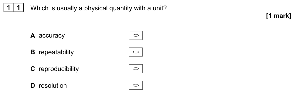
| Accuracy | How close a measurement is to the true value. |
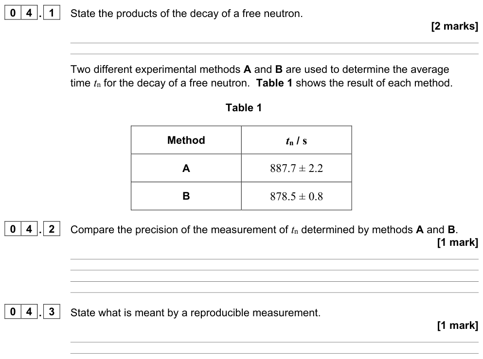
| Precision | How close repeated measurements are to each other (small spread). Precision depends only on random errors. |
| Repeatability | The same experimenter, using the same method and equipment, gets the same results. |
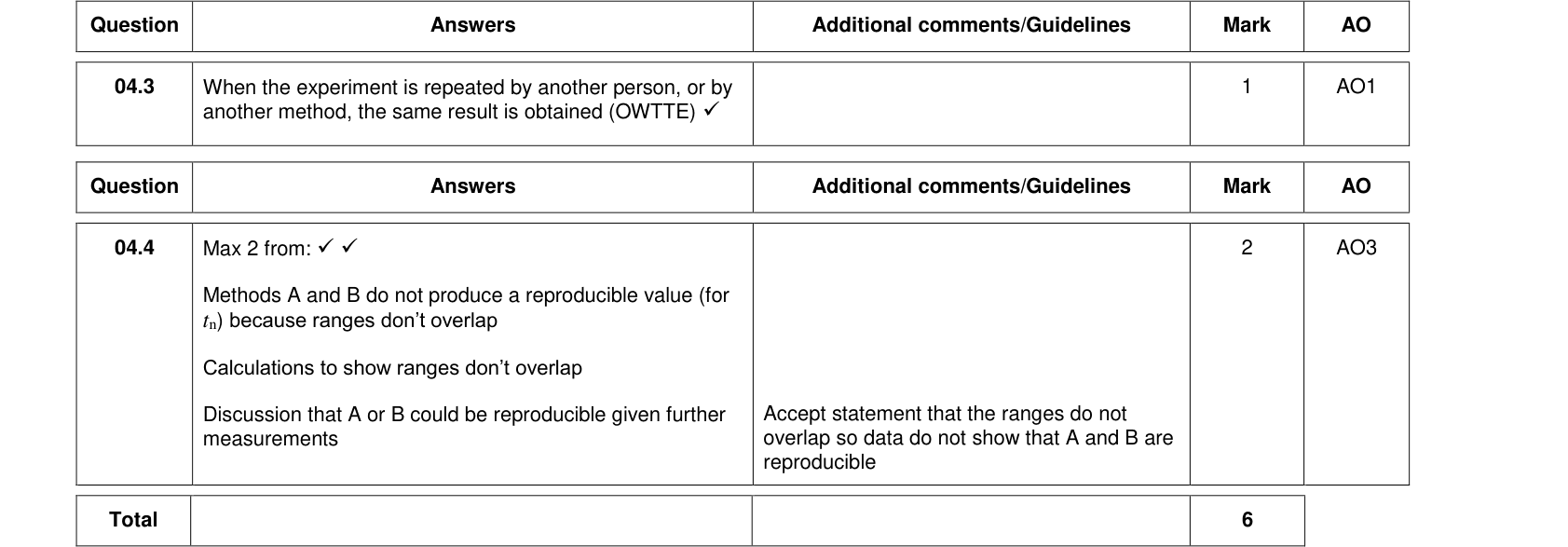
| Reproducibility | The same results are obtained by a different experimenter, or with a different method or different equipment. |
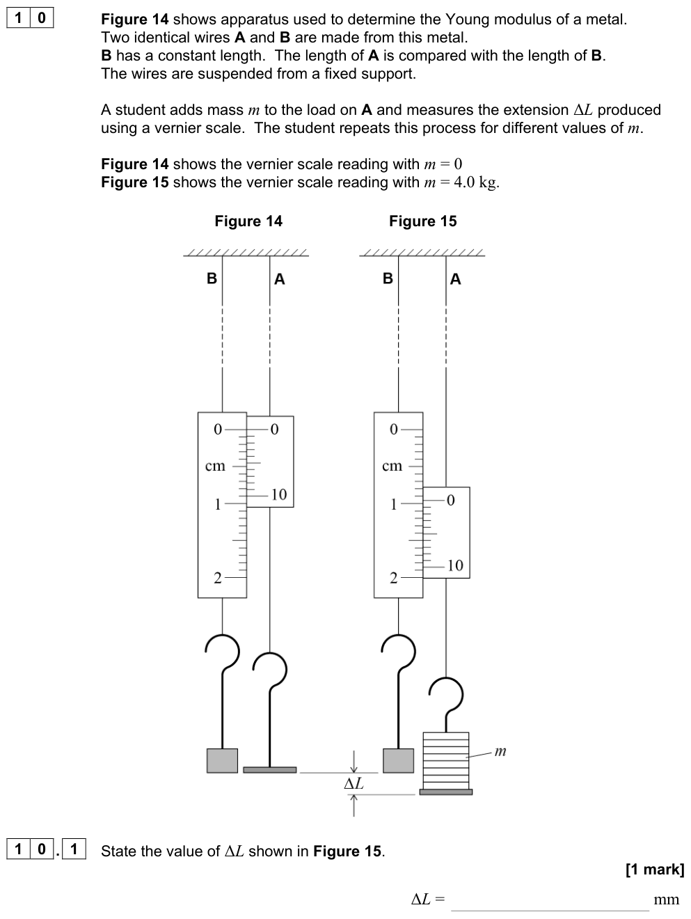
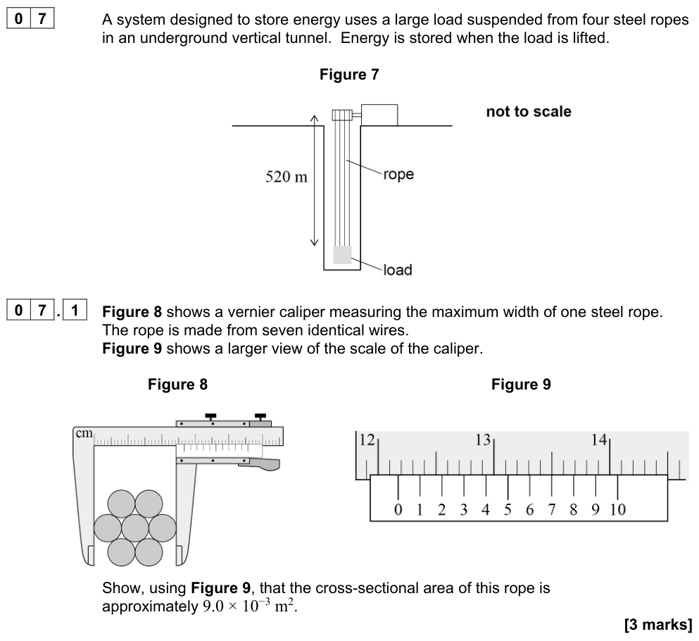
| Resolution | The smallest change in the quantity being measured that gives a perceptible change in the reading. A ruler marked in mm has a resolution of 1 mm; a micrometer has a resolution of 0.01 mm. |
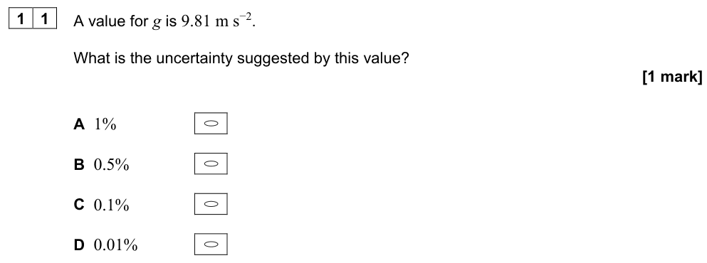
| Uncertainty | The interval within which the true value can be expected to lie, e.g. $l = 25.4 \pm 0.1\ \text{cm}$. |
Common mistake
Precise does not mean accurate. A set of readings can be tightly grouped (precise) but all wrong by the same amount because of a systematic error (inaccurate). Try the accuracy vs precision diagram in the Interactive tab.
Absolute, fractional and percentage uncertainty
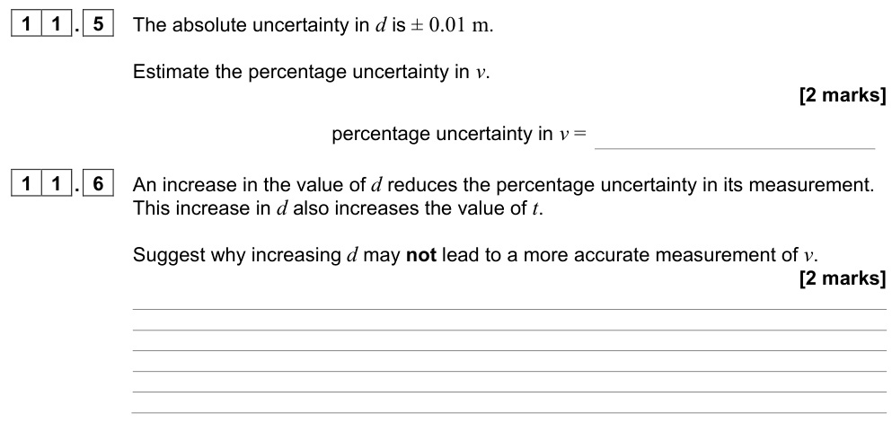
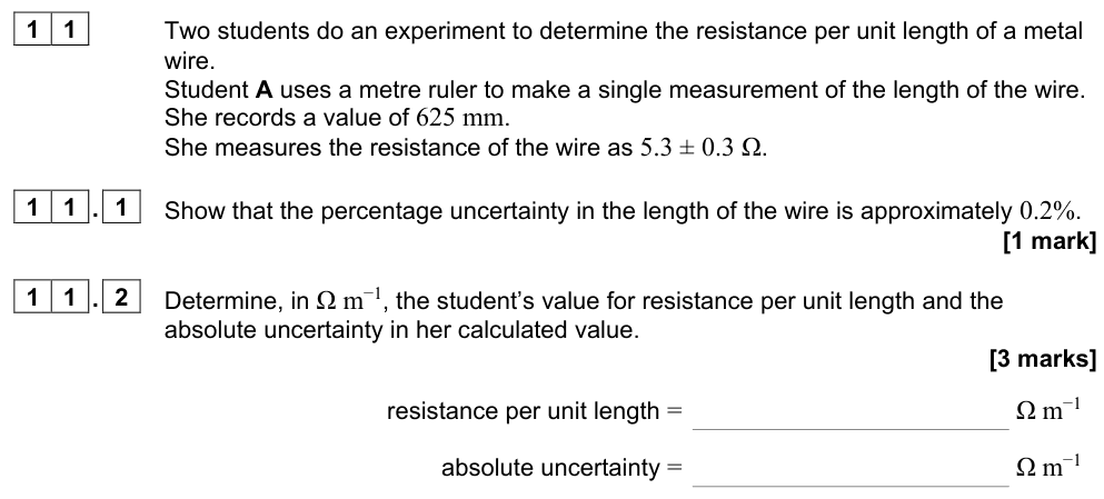
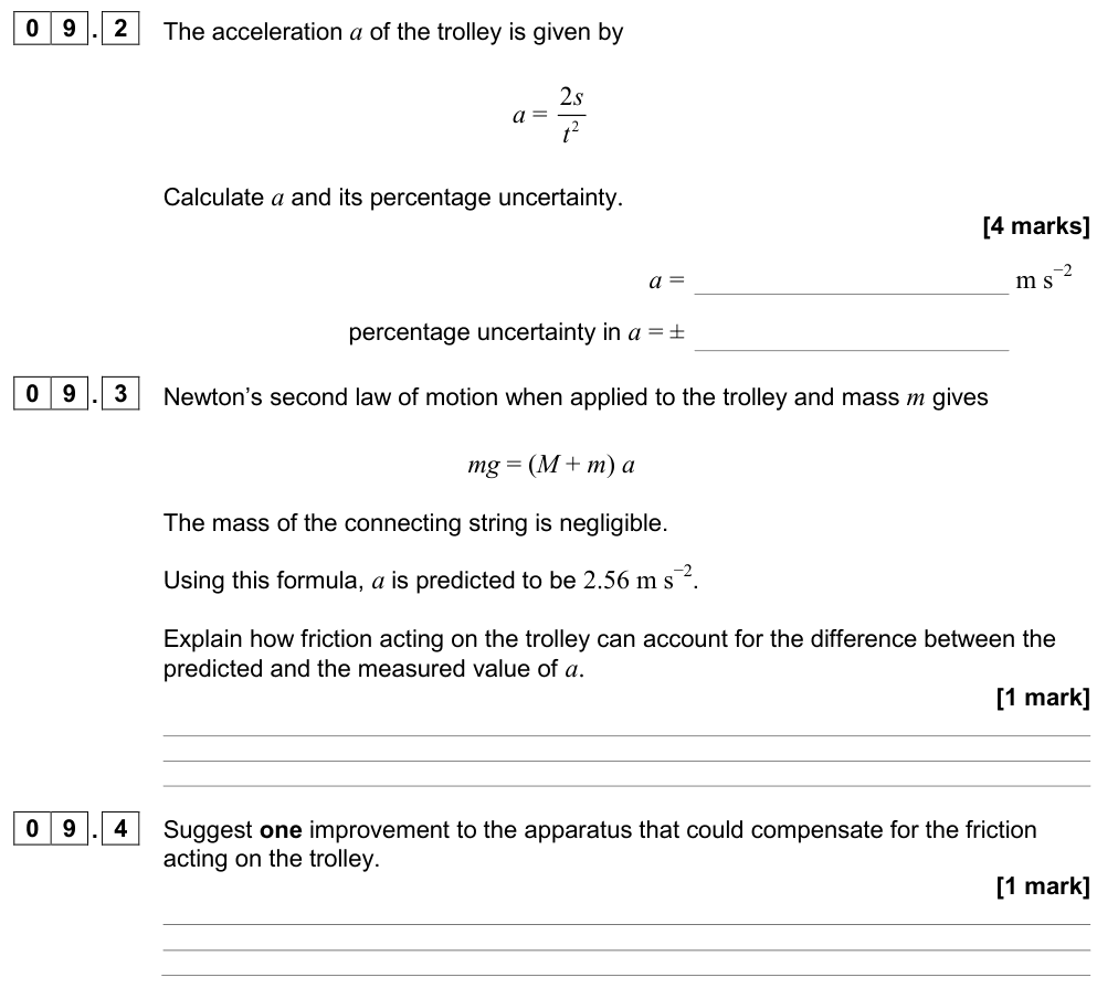
The absolute uncertainty $\Delta x$ has the same unit as the quantity. Writing $x \pm \Delta x$ means the true value is expected to lie between $x - \Delta x$ and $x + \Delta x$.
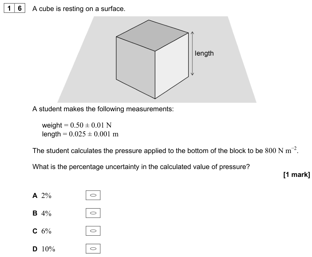
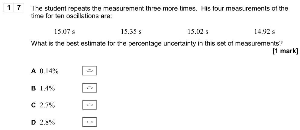
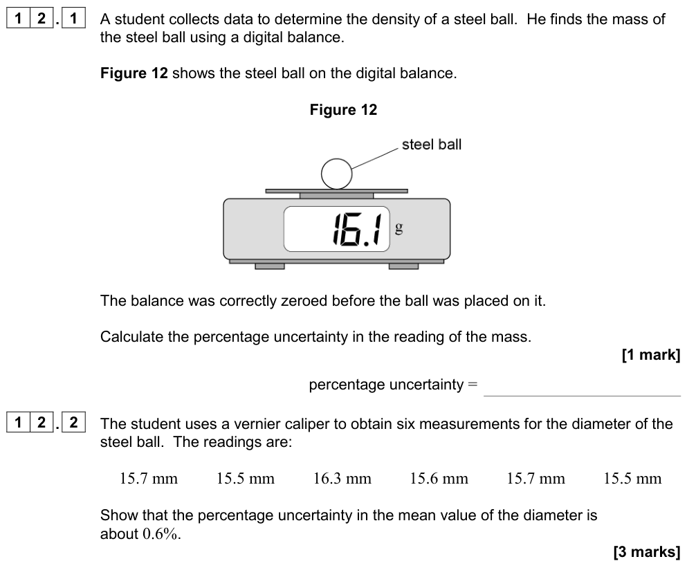
$$\text{fractional uncertainty} = \frac{\Delta x}{x} \qquad \text{percentage uncertainty} = \frac{\Delta x}{x} \times 100\%$$
Where does the uncertainty come from?
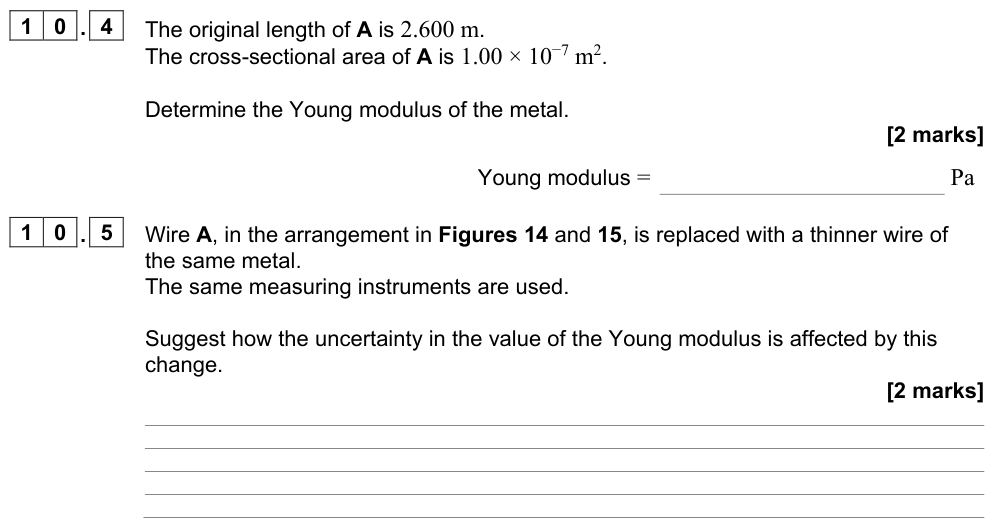
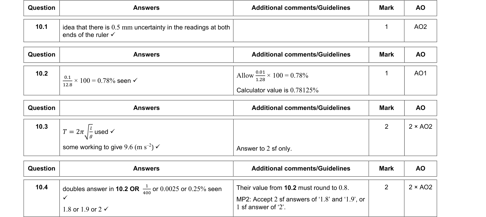
- A single reading on an analogue scale: $\pm$ half the smallest division (for example $\pm 0.5\ \text{mm}$ on a mm ruler for one reading).
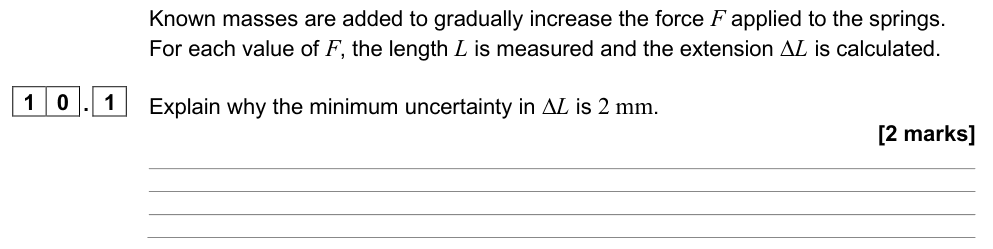
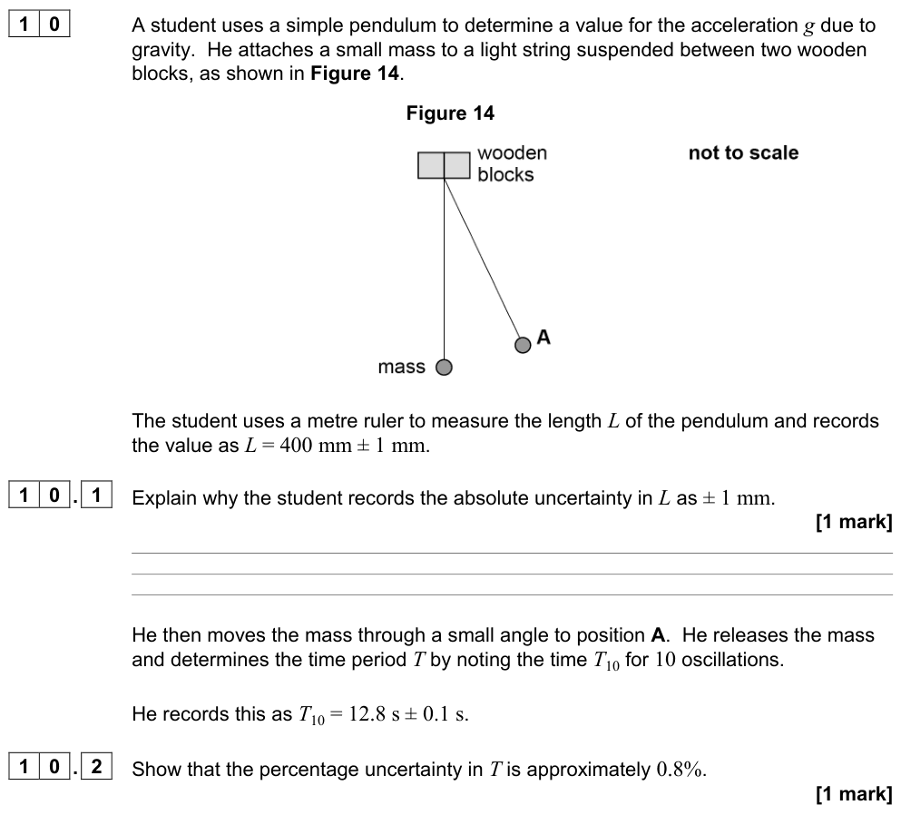
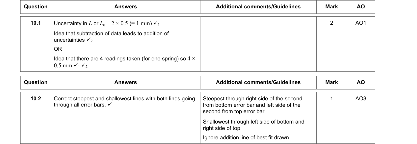
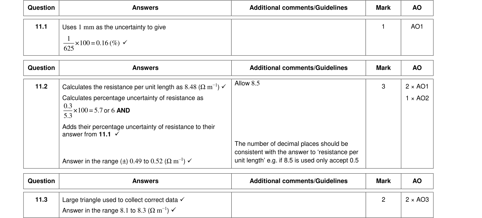
- A length found from two readings (both ends of a ruler): the uncertainty in each end adds, so $\pm 1$ smallest division ($\pm 1\ \text{mm}$).
- A digital meter: $\pm$ the resolution (the last digit), unless the manufacturer gives a larger value.
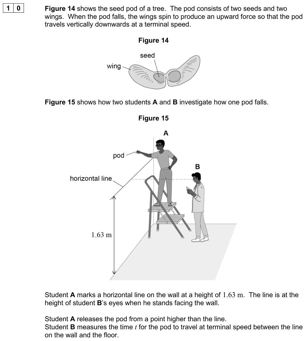
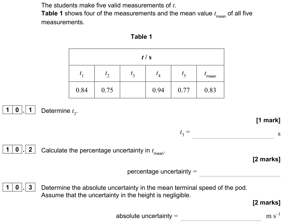
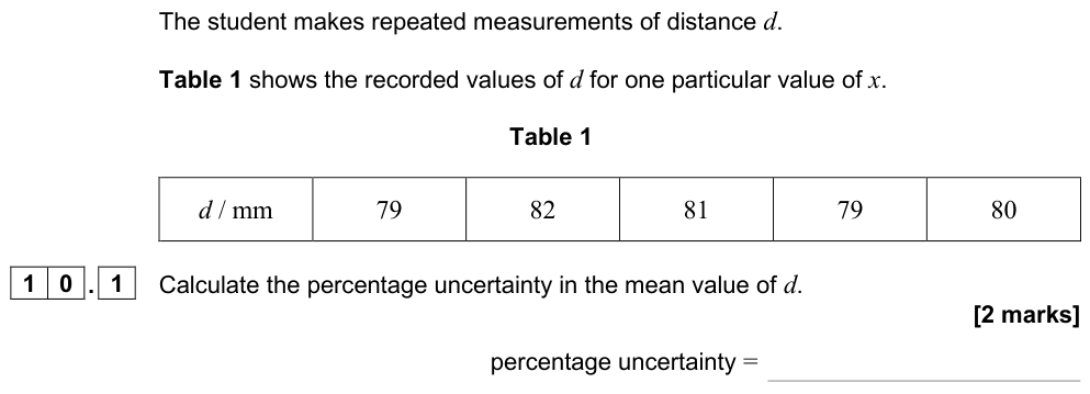
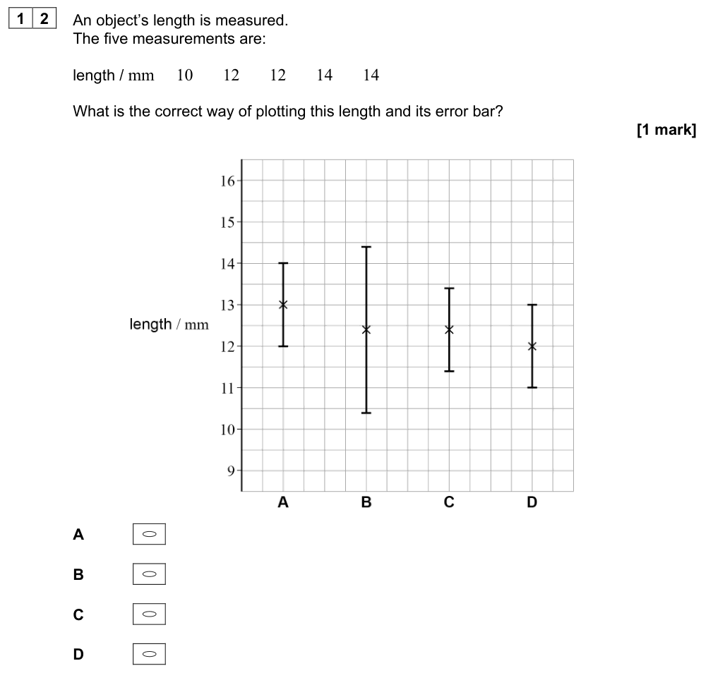
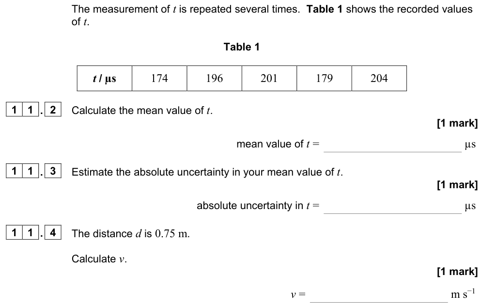
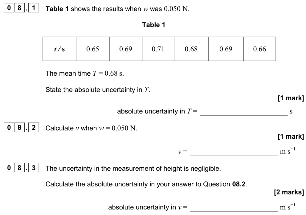
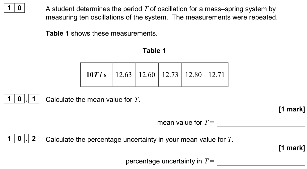
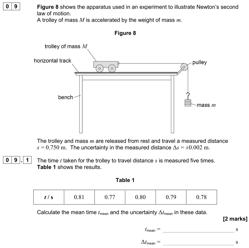
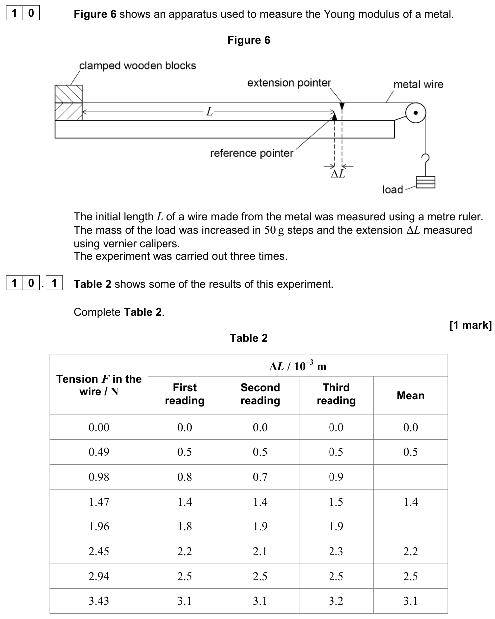
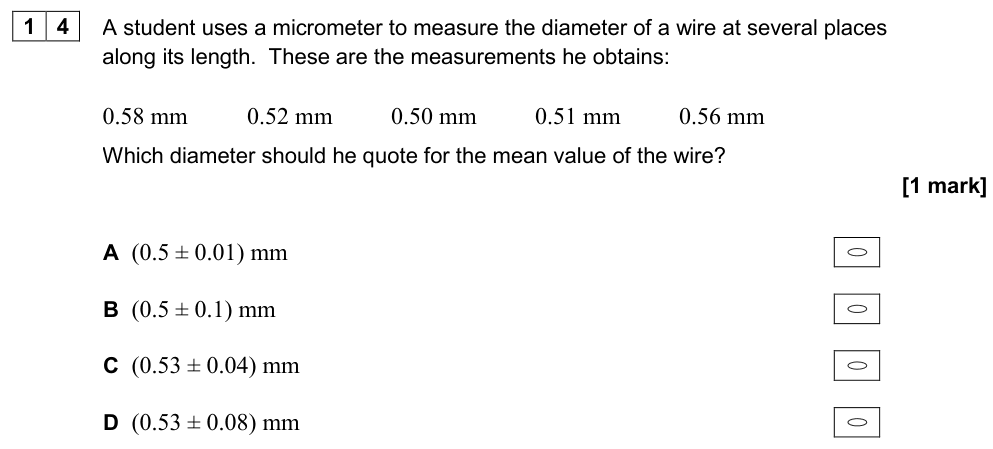
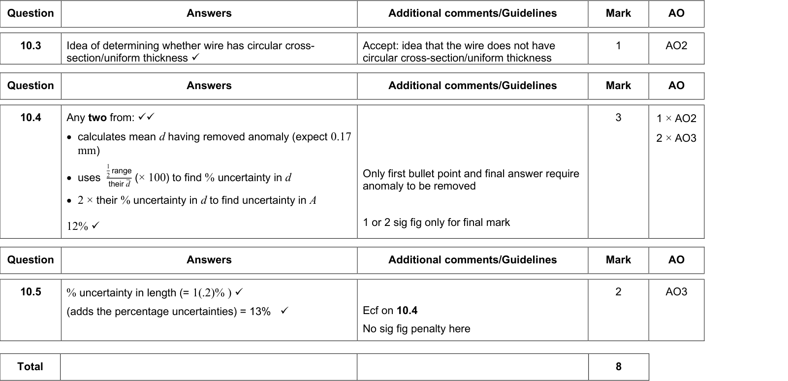
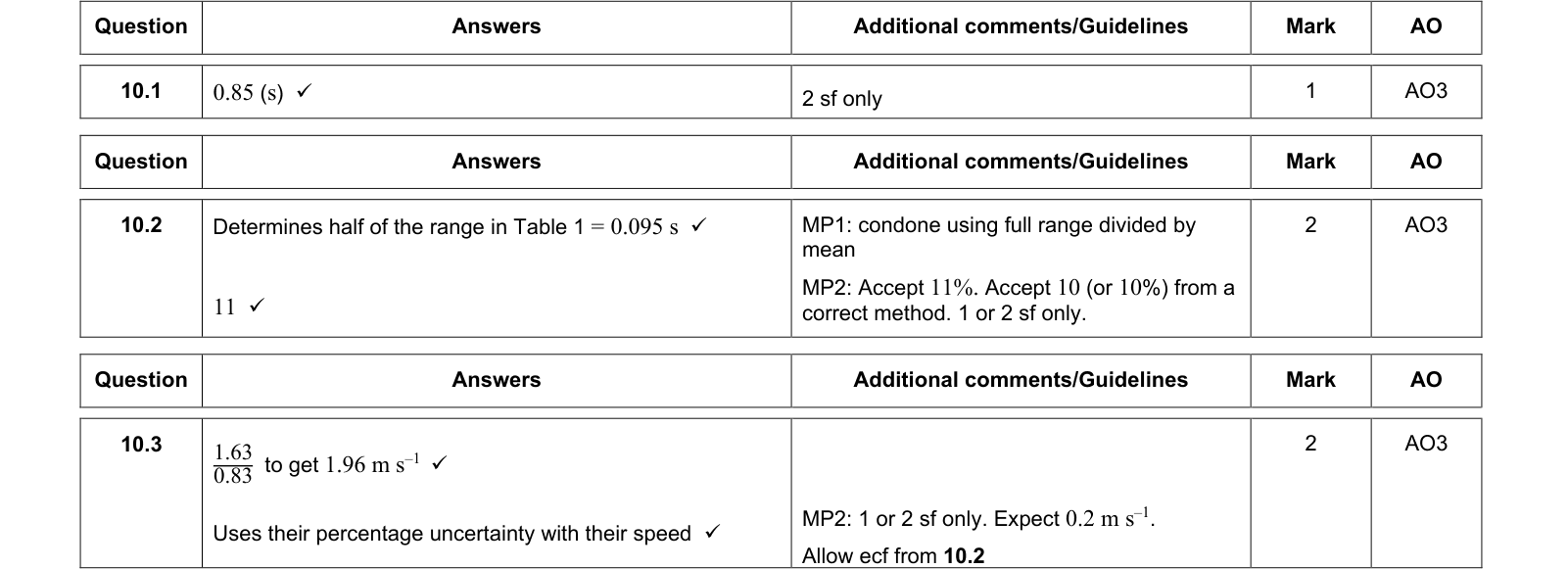
- Repeated readings: use the mean as the best value, and half the range as the uncertainty:
$$\Delta x = \frac{x_{\max} - x_{\min}}{2}$$
Worked example: repeated readings
Five readings of the time for 10 swings of a pendulum: 14.2 s, 14.5 s, 14.3 s, 14.6 s, 14.4 s.
Mean $= 14.4\ \text{s}$; range $= 14.6 - 14.2 = 0.4\ \text{s}$; uncertainty $= \pm 0.2\ \text{s}$.
Period $T = 14.4/10 = 1.44\ \text{s}$ with uncertainty $0.2/10 = \pm 0.02\ \text{s}$. Timing many swings makes the percentage uncertainty in $T$ ten times smaller.
Exam tip
Discard anomalous readings before calculating the mean, and say so. Then quote the mean to the same resolution as the readings.
Combining uncertainties
When you calculate a result from several measured values, the uncertainties combine using three rules.
Rules for combining uncertainties
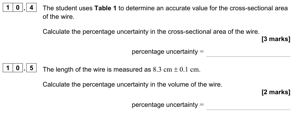
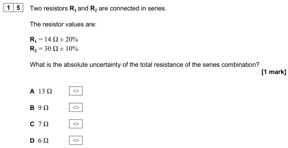
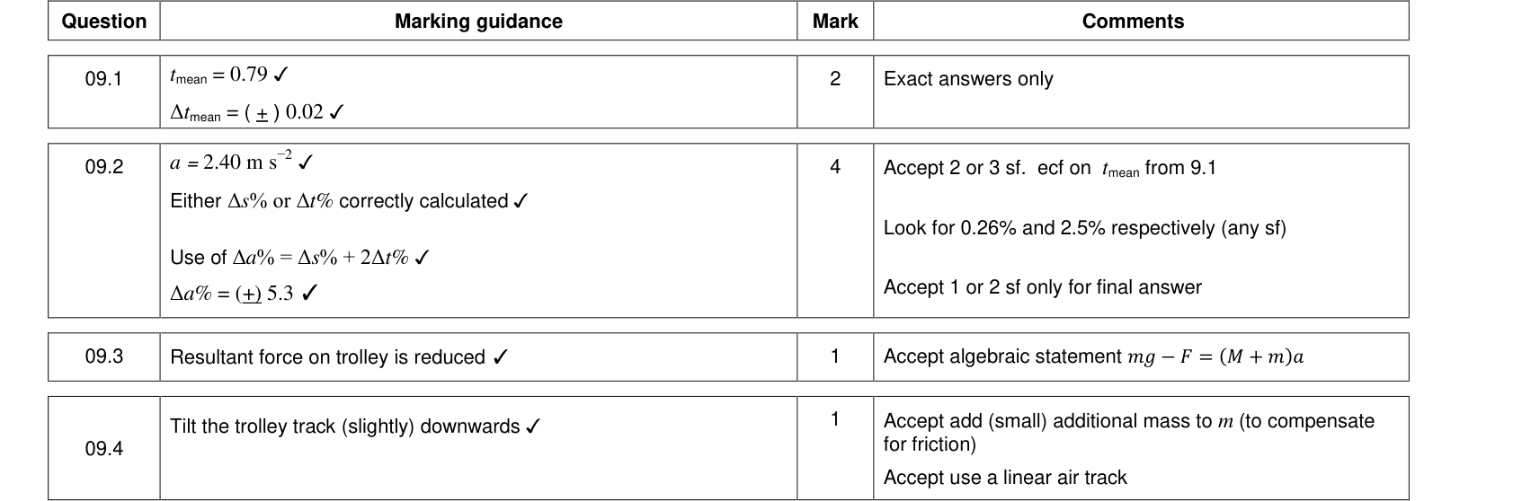
- Adding or subtracting quantities: add the absolute uncertainties. If $y = a + b$ or $y = a - b$, then $\Delta y = \Delta a + \Delta b$.
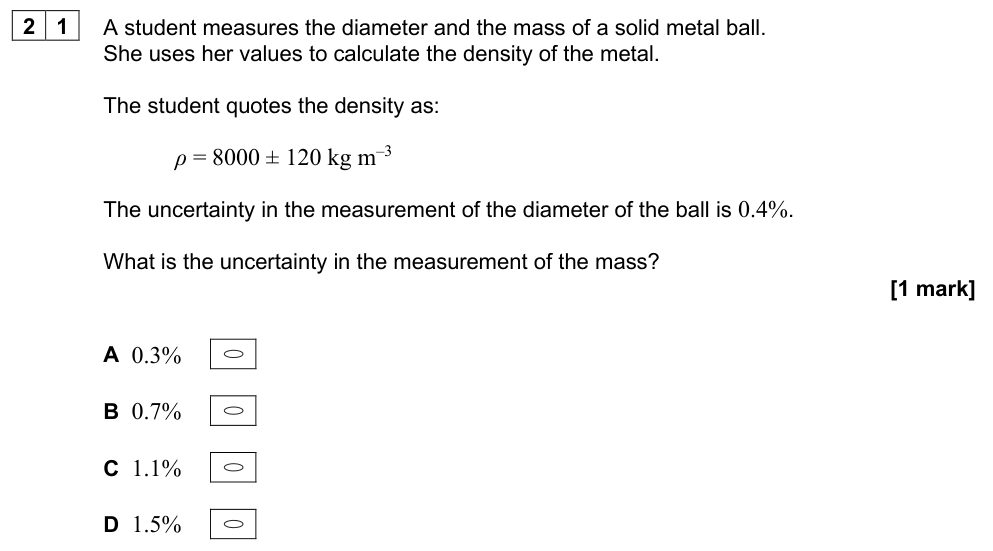
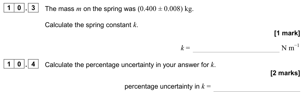
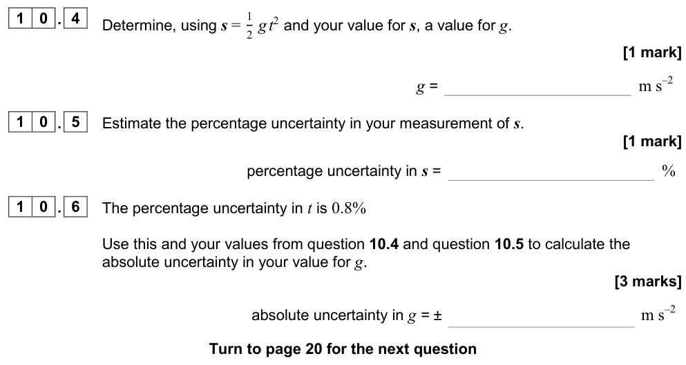
- Multiplying or dividing quantities: add the percentage (or fractional) uncertainties. If $y = ab$ or $y = a/b$, then $\%y = \%a + \%b$.
- Raising to a power: multiply the percentage uncertainty by the power. If $y = a^n$, then $\%y = |n| \times \%a$. (This includes square roots: $\sqrt{a}$ has half the percentage uncertainty of $a$.)
Constants such as $\pi$, $g$ (if given) and pure numbers have no uncertainty.
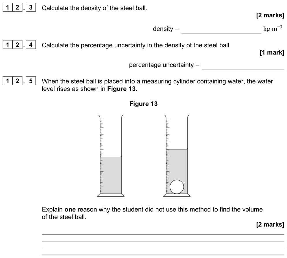
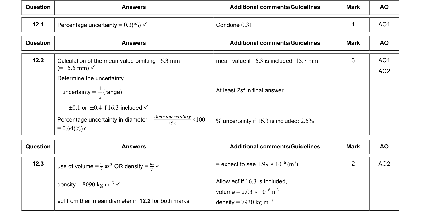
Worked example: density of a steel ball
Mass $m = 33.0 \pm 0.1\ \text{g}$, diameter $d = 20.0 \pm 0.1\ \text{mm}$.
$\%m = \dfrac{0.1}{33.0} \times 100 = 0.30\%$; $\%d = \dfrac{0.1}{20.0} \times 100 = 0.50\%$.
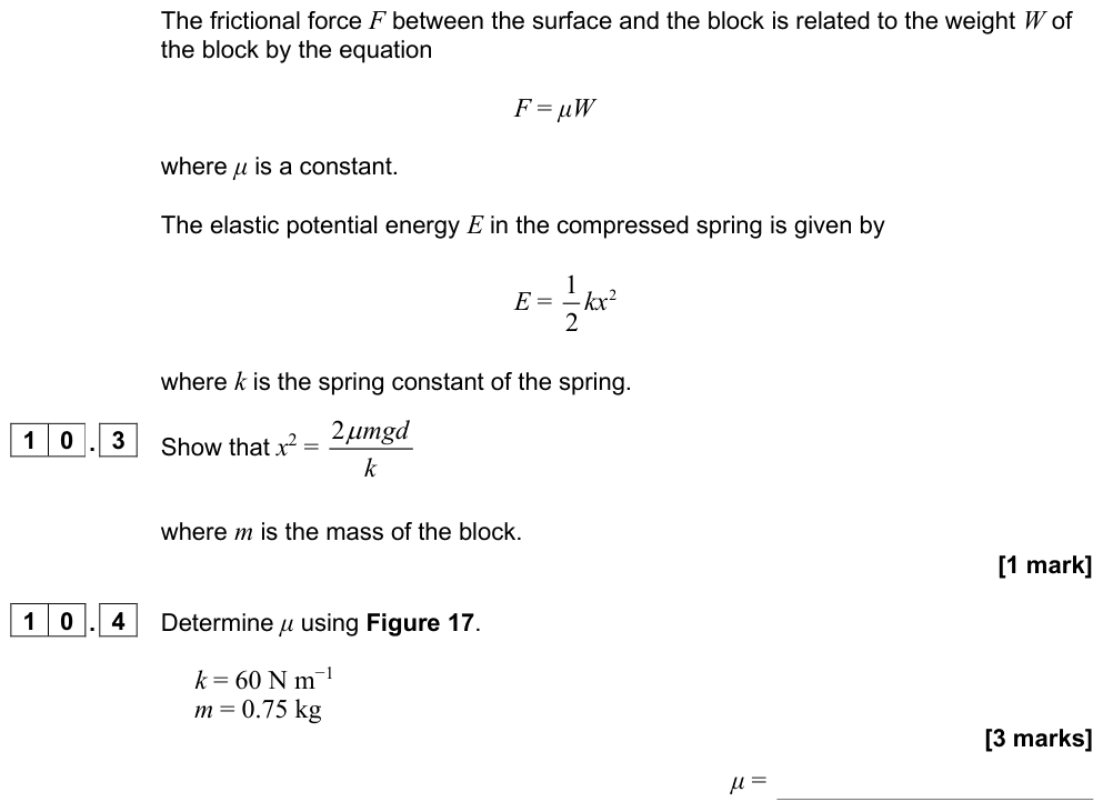
$\rho = \dfrac{m}{V} = \dfrac{m}{\frac{\pi}{6}d^3}$, so $\%\rho = \%m + 3 \times \%d = 0.30 + 1.5 = 1.8\%$.
$\rho = \dfrac{33.0 \times 10^{-3}}{\frac{\pi}{6}(20.0 \times 10^{-3})^3} = 7880\ \text{kg m}^{-3}$, so $\Delta\rho = 0.018 \times 7880 \approx 140\ \text{kg m}^{-3}$.
Result: $\rho = 7900 \pm 100\ \text{kg m}^{-3}$ (or $7880 \pm 140\ \text{kg m}^{-3}$).
Worked example: subtraction makes uncertainty worse
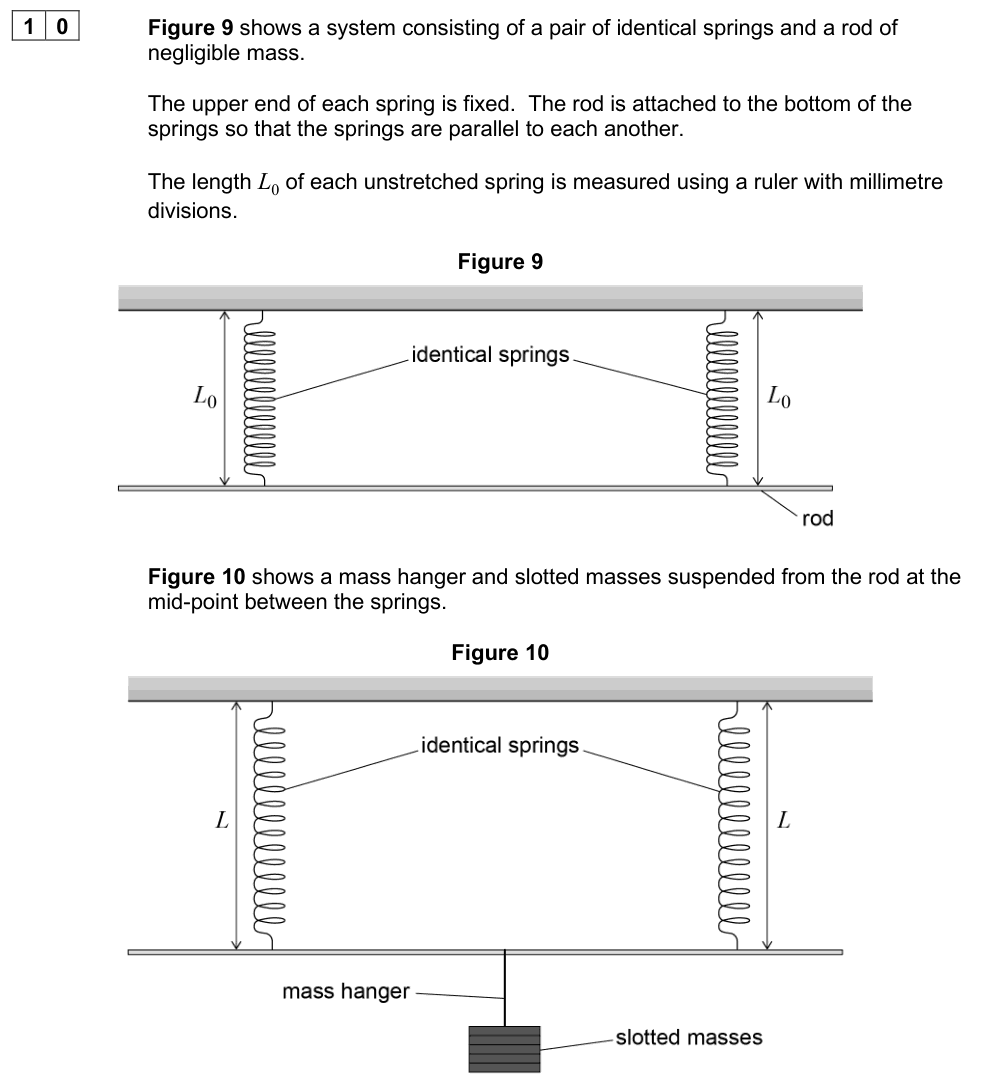
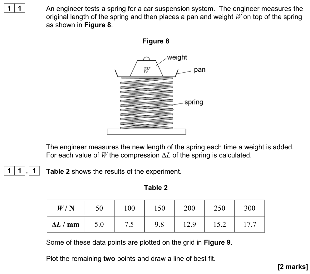
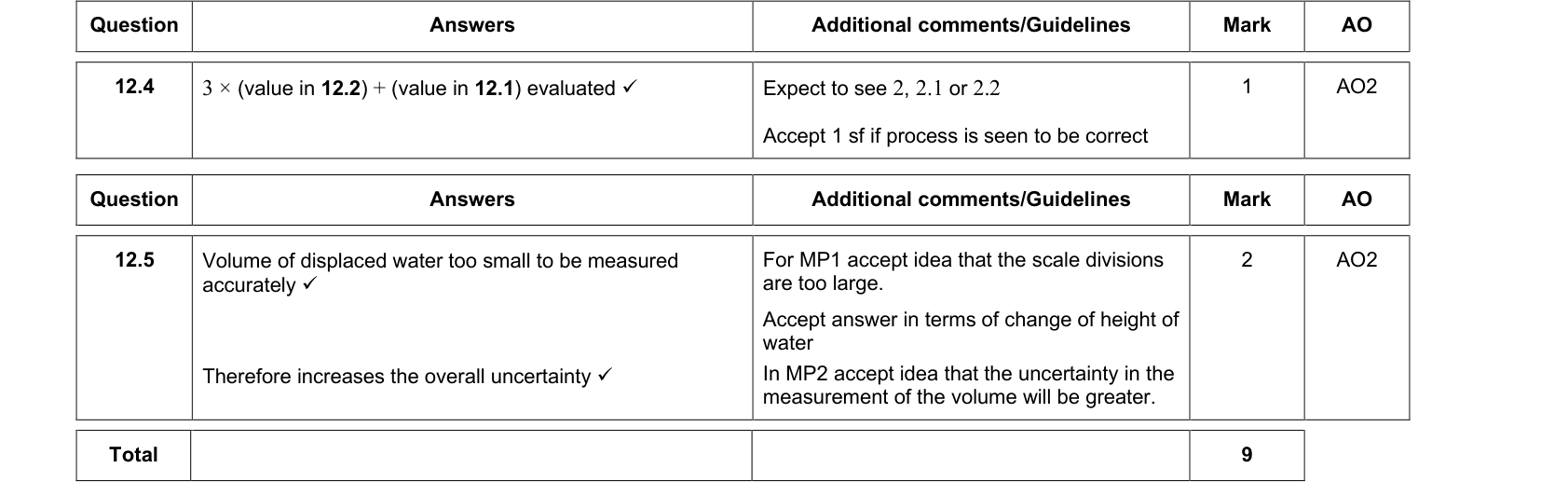
A spring is $15.0 \pm 0.1\ \text{cm}$ long unloaded and $16.2 \pm 0.1\ \text{cm}$ loaded. Extension $= 1.2 \pm 0.2\ \text{cm}$.
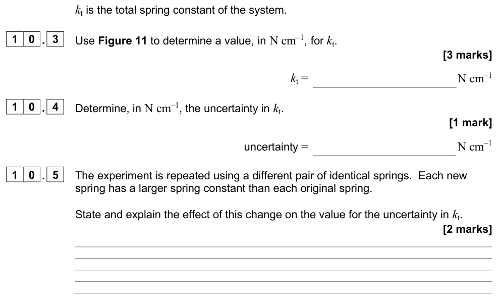
The readings each have about 0.7% uncertainty, but the extension has $0.2/1.2 = 17\%$. Small differences between large readings have large percentage uncertainties. Use a larger load or a more precise instrument.
Exam tip: which uncertainty dominates?
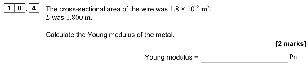
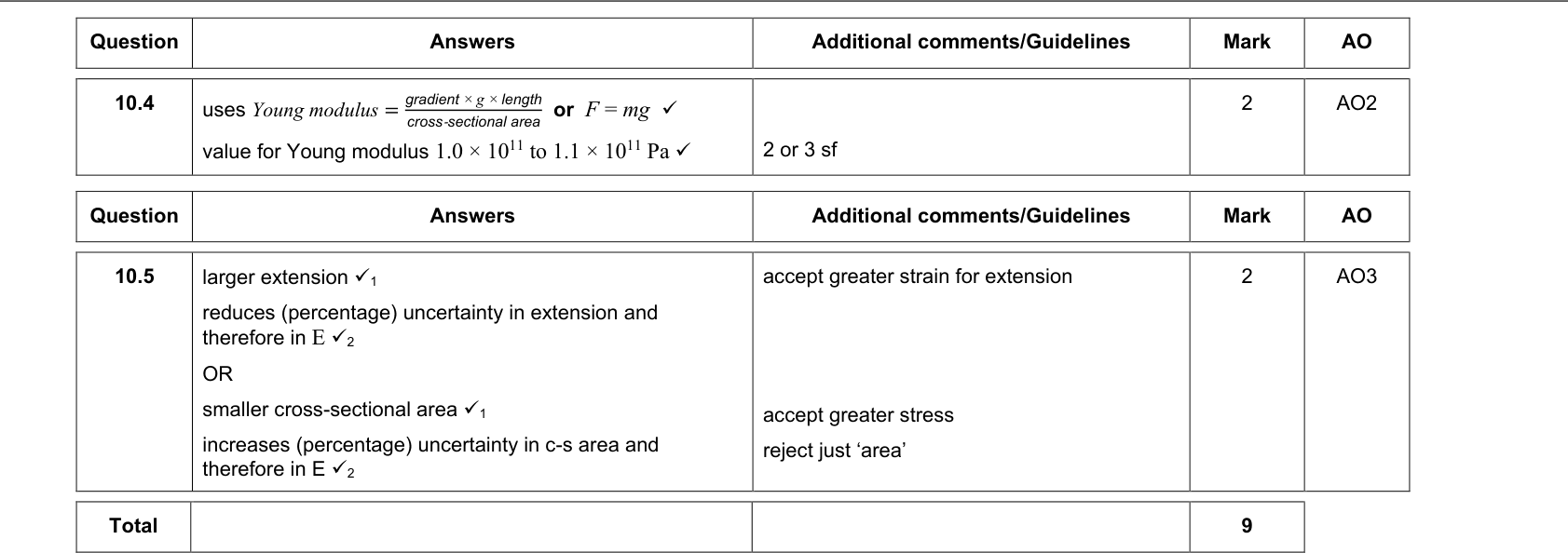
Questions often ask which measurement contributes most to the uncertainty. Compare percentage uncertainties, remembering to multiply by any power. A small diameter measured with a ruler (e.g. $0.5 \pm 0.1\ \text{mm}$ = 20%, squared → 40%) usually dominates. That is why the diameter of a wire is measured with a micrometer at several places and averaged.
Error bars and the uncertainty in a gradient
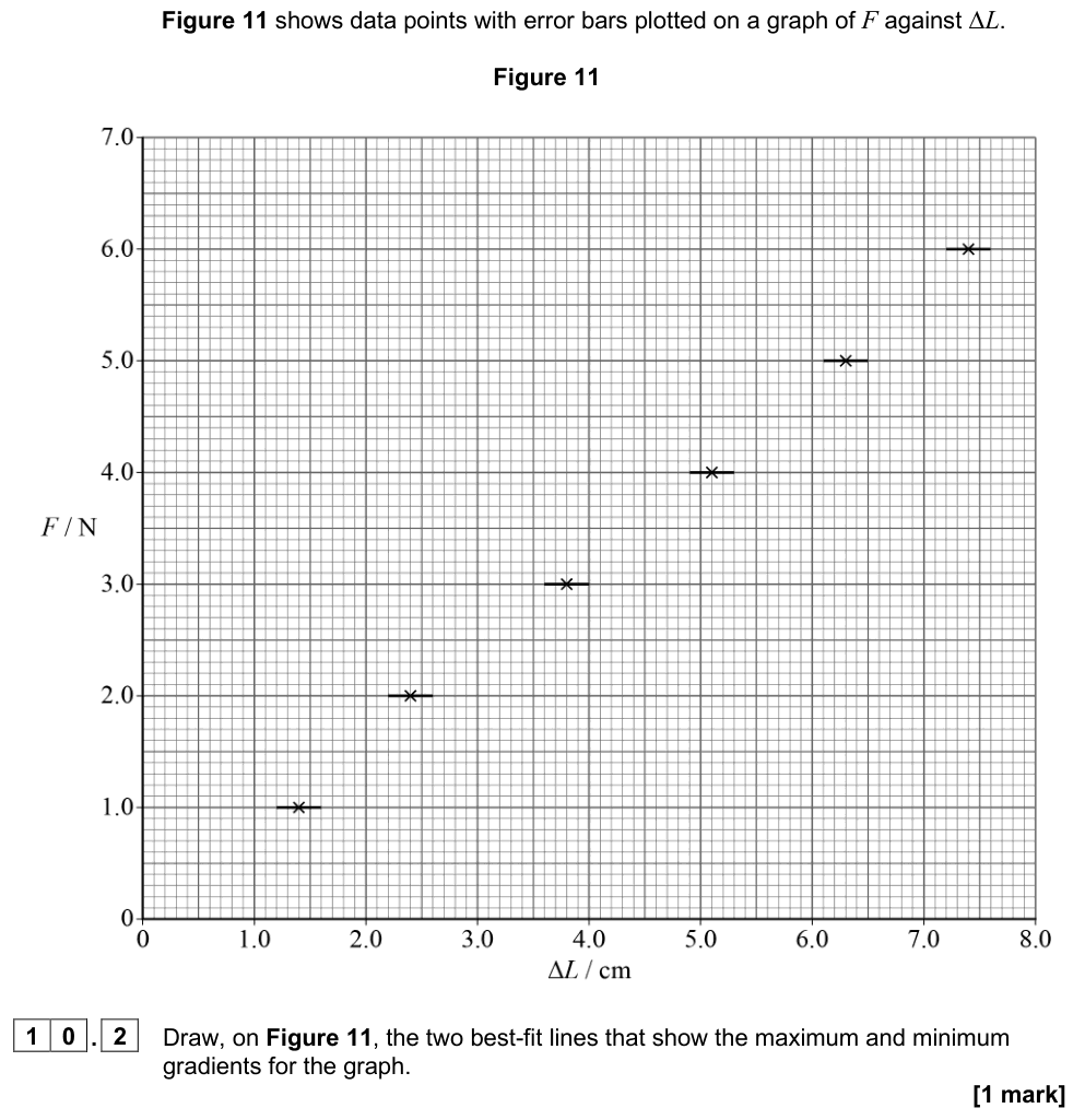
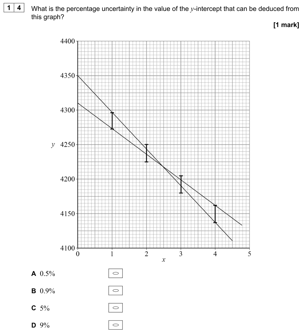
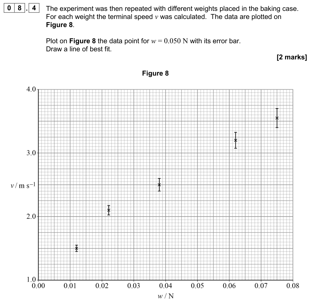
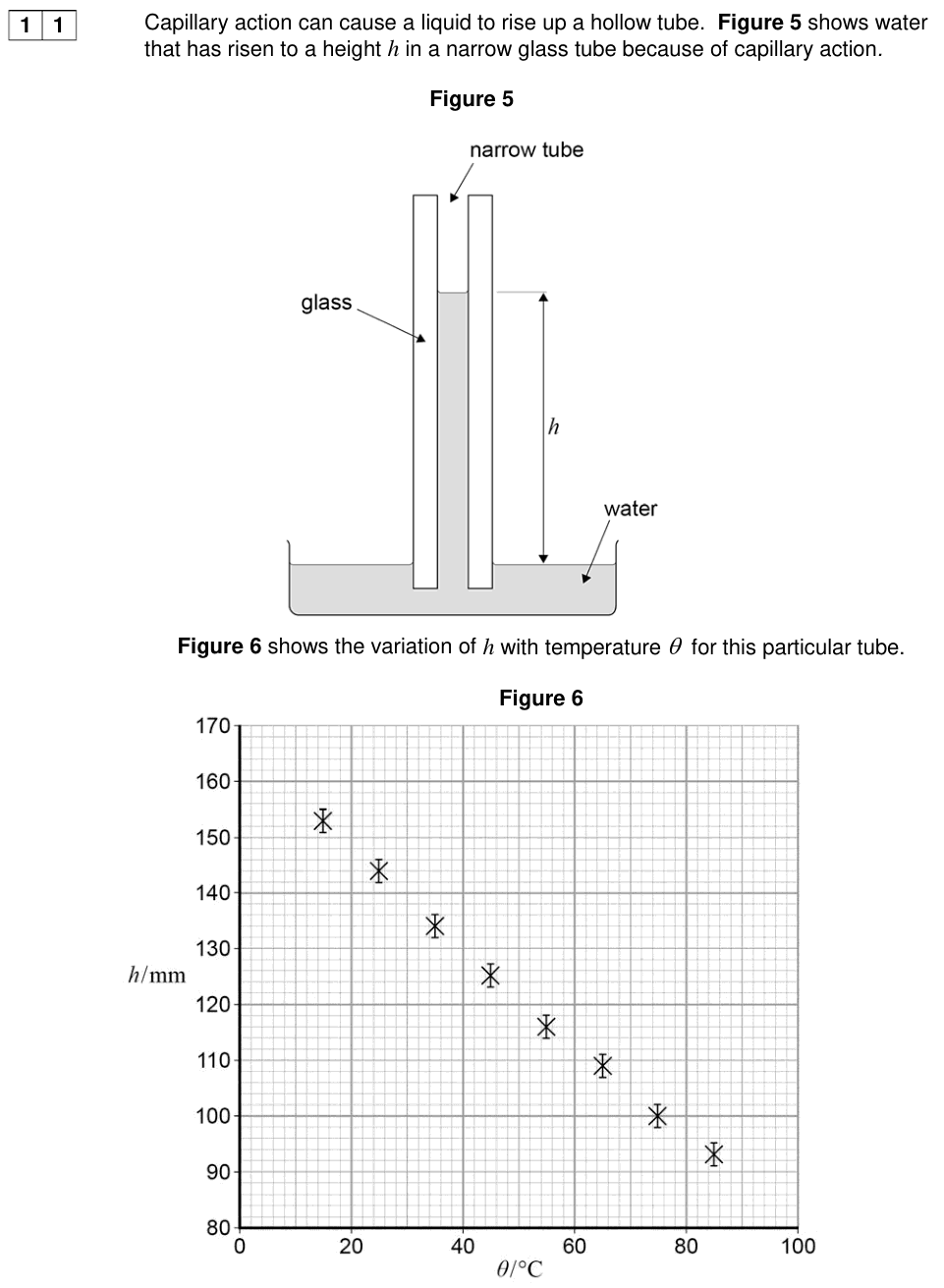
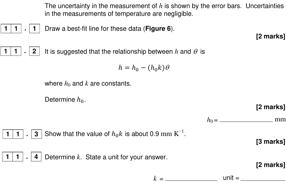
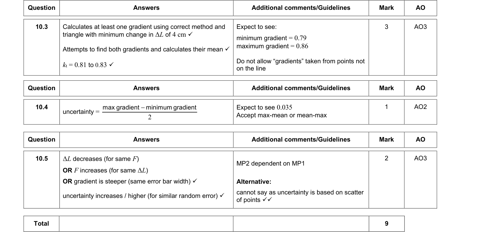
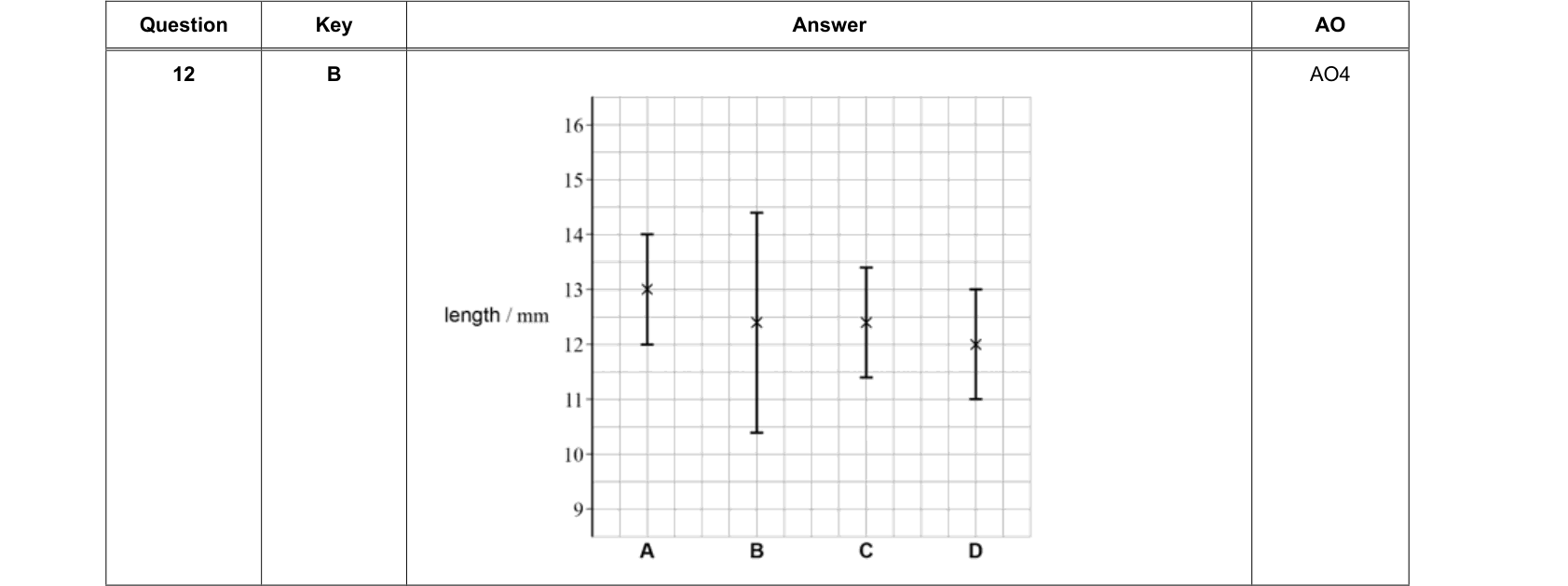
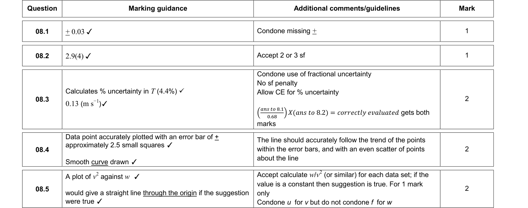
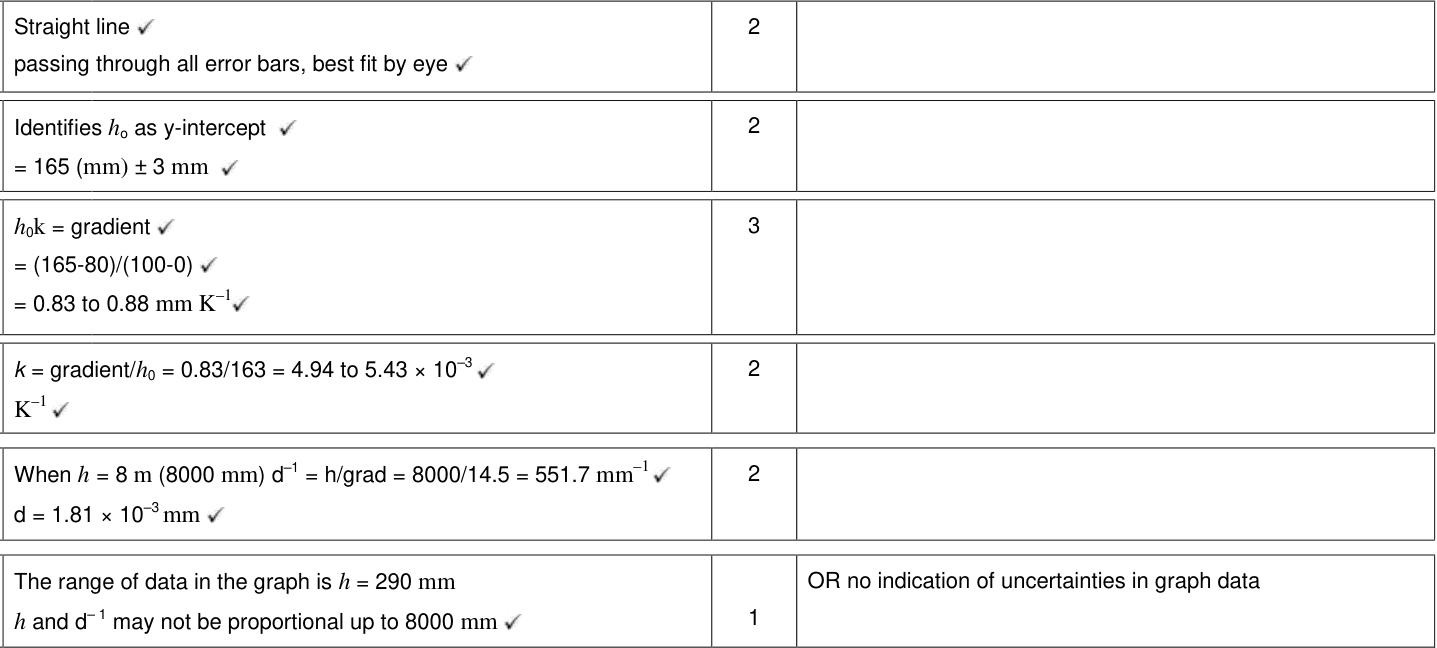
On a graph, the uncertainty in a data point is shown with an error bar: a line extending $\pm\Delta y$ (and/or $\pm\Delta x$) from the point. The total length of the bar is $2\Delta y$.
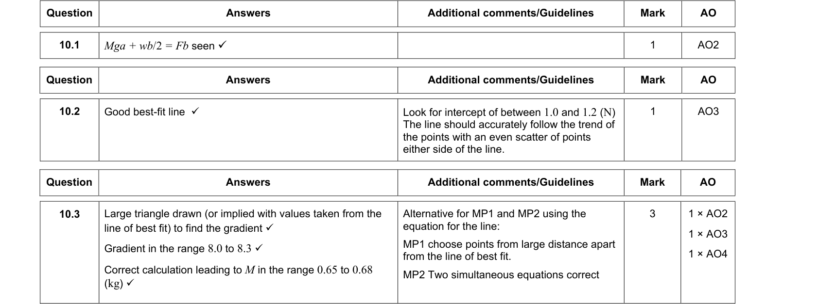
To find the uncertainty in a gradient:
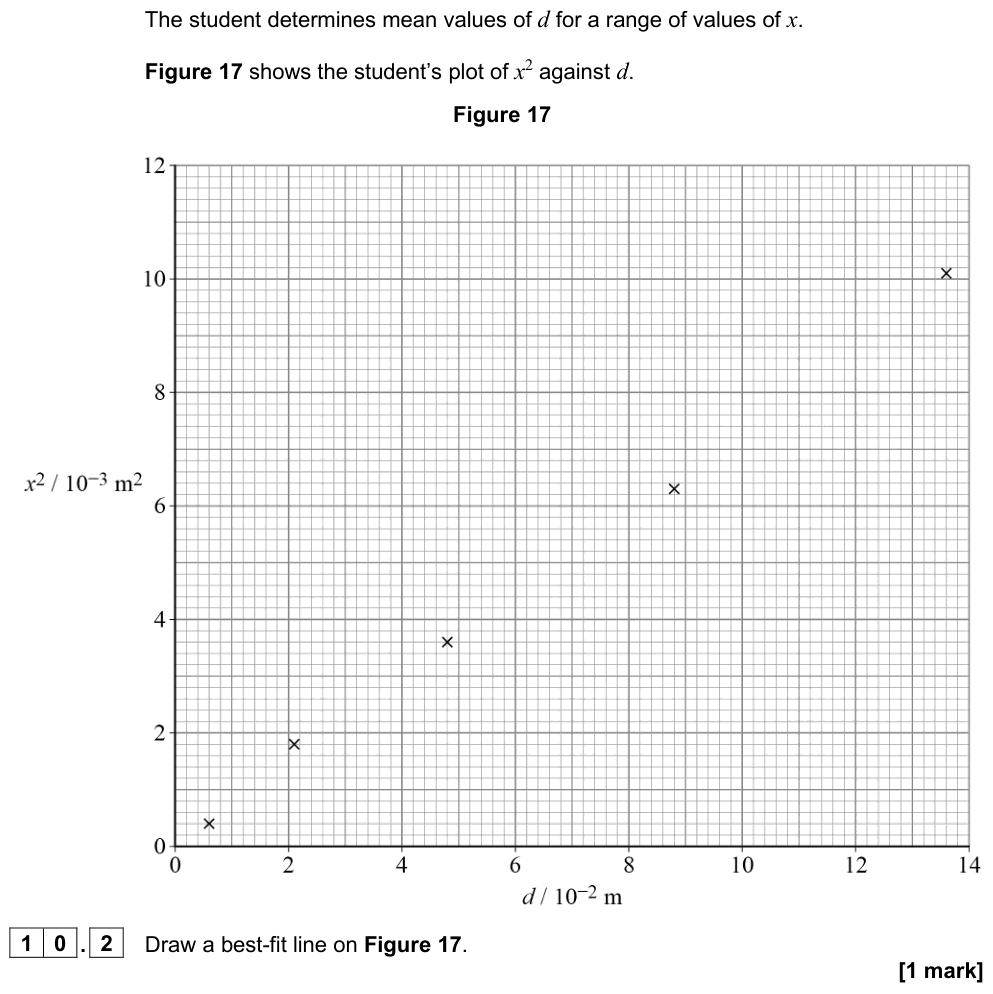
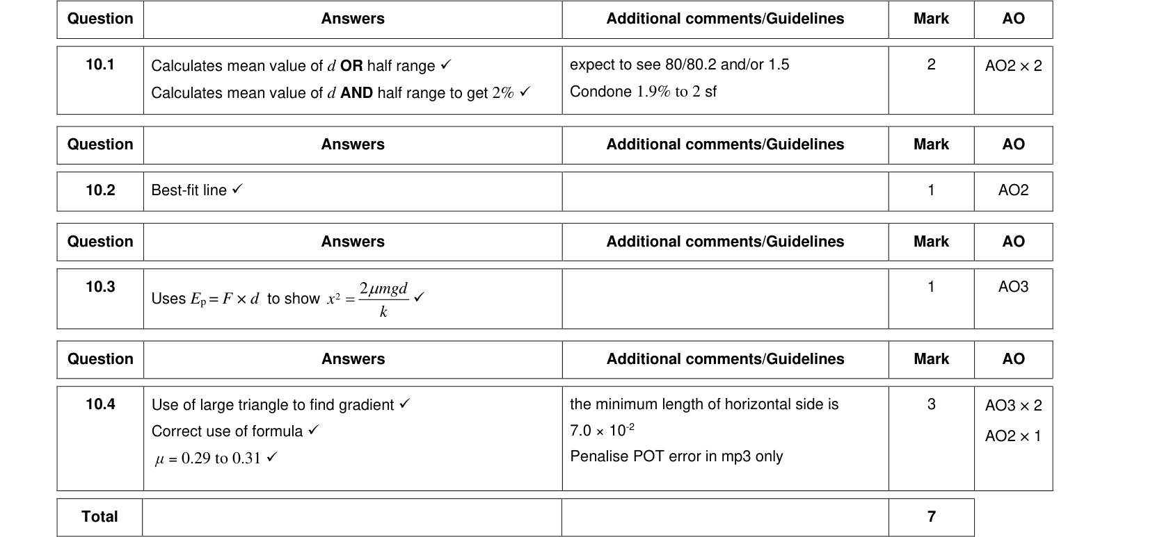
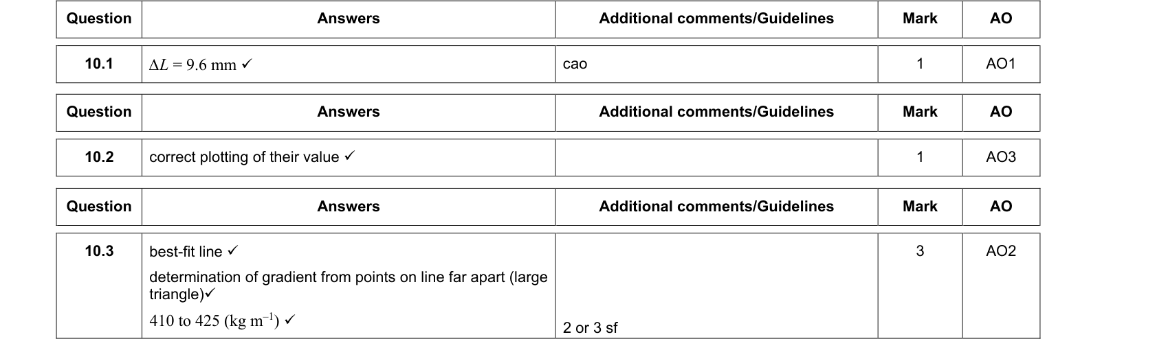
- Draw the line of best fit, with points evenly scattered either side.
- Draw the steepest and shallowest straight lines that still pass through all the error bars (the worst acceptable lines).
- Calculate the gradient of each line.
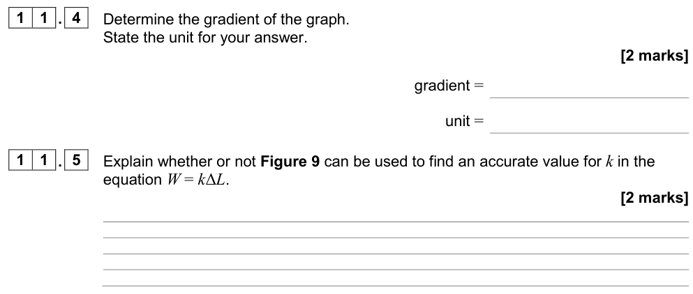
$$\Delta(\text{gradient}) = \frac{m_{\max} - m_{\min}}{2} \quad \text{or} \quad \Delta(\text{gradient}) = |m_{\text{best}} - m_{\text{worst}}|$$
$$\%\text{ uncertainty in gradient} = \frac{\Delta(\text{gradient})}{m_{\text{best}}} \times 100\%$$
The uncertainty in the intercept is found in the same way, from the intercepts of the best and worst lines.
Exam tip: drawing graphs
- Use more than half of the grid in both directions; choose scales of 1, 2 or 5 units per large square (never 3).
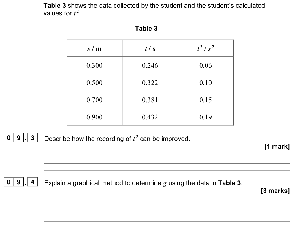
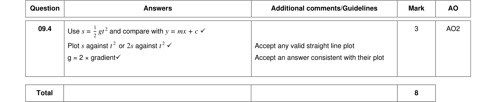
- Label axes with quantity and unit, e.g. $t^2\ /\ \text{s}^2$.
- Plot points to within half a small square; use small crosses.
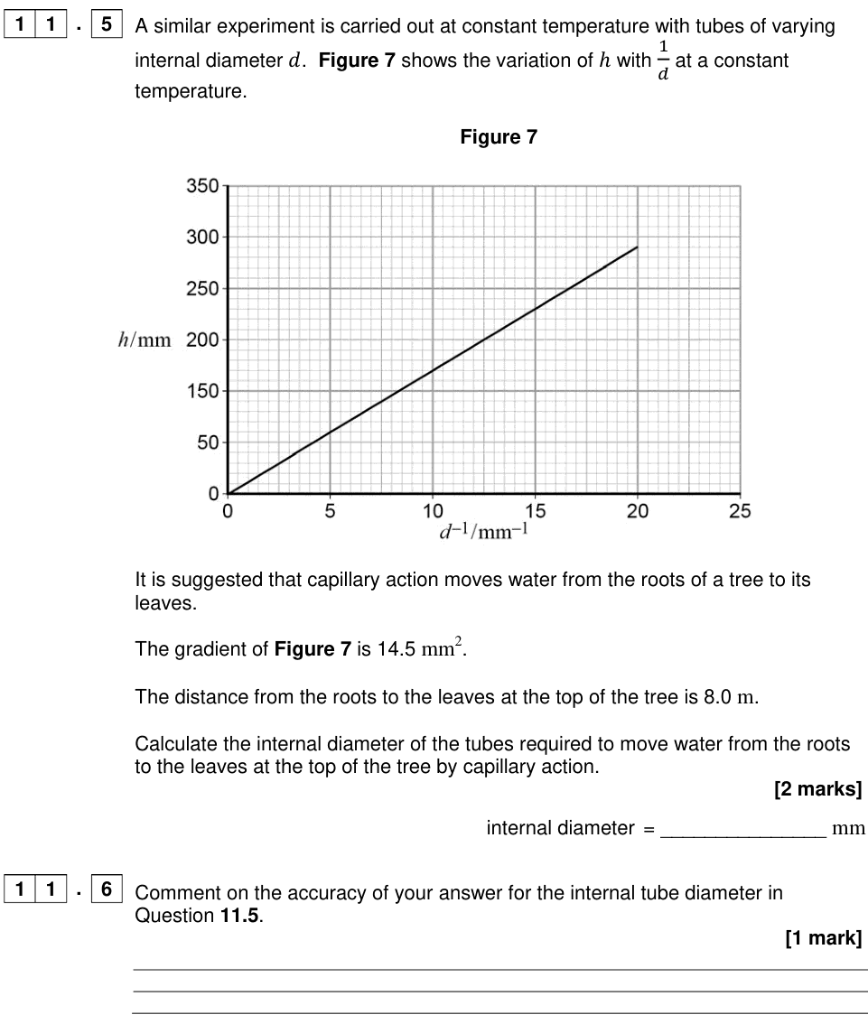
- When calculating a gradient, use a large triangle (at least half the line) and read points that lie on the line, not data points.
The gradient uncertainty diagram in the Interactive tab lets you drag the worst lines and see how the gradient uncertainty changes.
Significant figures and quoting results
- Quote the uncertainty to 1 (or at most 2) significant figures.
- Quote the value to the same decimal place as the uncertainty: $9.79 \pm 0.06\ \text{m s}^{-2}$, not $9.7854 \pm 0.06$.
- The number of significant figures in data indicates its precision: $2.50\ \text{m}$ implies a resolution of 0.01 m.
Comparing with an accepted value
$$\%\text{ difference} = \frac{|\text{experimental value} - \text{accepted value}|}{\text{accepted value}} \times 100\%$$
If the percentage difference is smaller than the percentage uncertainty, the result agrees with the accepted value within experimental uncertainty. If it is larger, there is probably a systematic error that the uncertainty analysis has not accounted for.
Summary
- Random errors scatter readings; reduce them by repeating and averaging. Systematic errors shift every reading; remove them by recalibrating or improving technique.
- Accuracy is closeness to the true value; precision is closeness of repeated readings to each other.
- Add absolute uncertainties for $+$ and $-$; add percentage uncertainties for $\times$ and $\div$; multiply by $n$ for powers.
- Gradient uncertainty: compare best-fit and worst acceptable lines through the error bars.